Asset Pricing [Part 2b : Sketching The Traditional Framework]

According to the Two-fund separation theorem of Modern Portfolio Theory, the investment problem can be decomposed into the following steps:

1. Finding the optimal portfolio of risky assets
2. Finding the best combination of this optimal risky portfolio and the risk free asset.

This post will concentrate on the second issue first. The problem of finding an optimal risky portfolio will be addressed in the next post.

[The Capital Allocation Line]

To simplify the procedure for finding the optimal combination of the risk free and the risky funds, one can first consider the return on a portfolio consisting of one risky asset and a risk free asset. The return on such a portfolio is simply:

The variance of this combined portfolio is given by:

These two results can be combined to yield the following expression :

This is the Capital Allocation Line (CAL) and represents the set of investment possibilities created by all combinations of the risky and riskless asset. The price of risk is the return premium per unit of portfolio risk and depends only on the prices of available securities. This ratio is also known as the Sharpe ratio. To illustrate how the CAL works, let us first set up some functions to [a] simulate random asset returns from a normal distribution and [b] calculate and draw the CAL connecting one risky asset with the risk free rate. These functions correspond to simulate.assets,CAL.line and DrawCAL as shown below.

#############################################################################
#
# Simulate asset returns from a normal distribution
#
#############################################################################

simulate.assets <- function(num.assets){
	ret.matrix <- matrix(dimnames=list(c(seq(1,100)),c(paste('Asset',1:num.assets))),(rep(0,num.assets*100)),nrow=100,ncol=num.assets,byrow=FALSE)
	shock <- matrix(dimnames=list(c(seq(1,100)),c(paste('Asset',1:num.assets))),(rep(0,num.assets*100)),nrow=100,ncol=num.assets,byrow=FALSE)
	for(i in 1:num.assets){
    	ret.matrix[,i]=rnorm(100,mean=runif(1,-0.8,0.2),sd=runif(1,0.8,2))
	    shock[,i] <- rnorm(100,colMeans(ret.matrix)[i],apply(ret.matrix,2,sd)[i])
	}
	sd.matrix <- apply(ret.matrix,2,sd)
	var.matrix <- var(ret.matrix)
	risk.free <- 0.02
	mean.ret <- colMeans(ret.matrix)
	sim.assets <- list(ret.matrix,var.matrix,sd.matrix,risk.free,mean.ret,shock)
	return(sim.assets)
}

 

#############################################################################
#
# Capital Allocation Line
#
#############################################################################

CAL.line <- function(type,risky.assets,optimised.portfolio){

	if(type=='Assets' && is.null(risky.assets)==FALSE){
    	num.assets <- ncol(risky.assets[[1]])
	    asset.returns <- colMeans(risky.assets[[1]])
	    asset.risk <- risky.assets[[3]]

	} else if (type=='Sharpe' && is.null(optimised.portfolio)==FALSE){
	    num.assets <- 1
	    asset.returns <- optimised.portfolio[[4]][1]
	    asset.risk <- optimised.portfolio[[4]][2]
	}

	total.risk <- seq(0,2,by=0.01)
	risk.free <- risky.assets[[4]]

	CAL.complete <- vector('list',num.assets)
	price.risk <-c()
	total.return <-matrix(rep(0,length(total.risk)*num.assets),nrow=length(total.risk),ncol=num.assets)

	 for(i in 1:num.assets){
	 	price.risk[i] <- (asset.returns[[i]]-risk.free)/asset.risk[i]
	    total.return[,i] <- risk.free+(price.risk[i]*total.risk)
	 	CAL.complete[[i]]<-cbind(total.risk,total.return[,i])
	 	colnames(CAL.complete[[i]]) <- c('Total Risk','Total Return')
	}
return(CAL.complete)
}

 

#############################################################################
#
# Draw Capital allocation Line (s)
#
#############################################################################

DrawCAL<-function(CAL,risky.assets,optimised.portfolio,legend.draw){

	num.lines <- length(CAL)
	num.assets <- ncol(risky.assets[[1]])
	plot.x.max <- max(risky.assets[[3]])+0.2
	plot.y.min <- min(risky.assets[[5]])-1
	plot.y.max <- max(risky.assets[[5]])+1

	windows()
	par(xaxs="i", yaxs="i")

	if(num.lines==1 && is.null(optimised.portfolio)==FALSE){
	  plot(xlab='Standard Deviation',ylab='Expected Return',ylim=c(plot.y.min,plot.y.max),xlim=c(0,plot.x.max),CAL[[1]],col='red',type='l',main='Capital Allocation Line',cex.main=0.85,cex.lab=0.75,cex.axis=0.75,lwd=2)
	  points(x=optimised.portfolio[[4]][2],y=(optimised.portfolio[[4]][1]),type='p',pch=9,col='dark blue',cex=1)
	} else if(num.lines==1 && is.null(optimised.portfolio)==TRUE){
	   plot(xlab='Standard Deviation',ylab='Expected Return',ylim=c(plot.y.min,plot.y.max),xlim=c(0,plot.x.max),CAL[[1]],col='red',type='l',main='Capital Allocation Line',cex.main=0.85,cex.lab=0.75,cex.axis=0.75,lwd=2)
	} else if(num.lines>1){
	   plot(xlab='Standard Deviation',ylab='Expected Return',ylim=c(plot.y.min,plot.y.max),xlim=c(0,plot.x.max),CAL[[1]],col='red',type='l',main='Capital Allocation Line',cex.main=0.85,cex.lab=0.75,cex.axis=0.75,lwd=2)
	   for(i in 2:num.lines){
	      lines(CAL[[i]],col='red',type='l',lwd=2)
	    }
	}
	points(x=0.01,y=risky.assets[[4]],type='p',pch=15,col='dark green',cex=1)
    points(x=risky.assets[[3]],y=risky.assets[[5]],type='p',pch=17,col='blue',cex=0.75)
    text(labels=1:num.assets,x=risky.assets[[3]],y=risky.assets[[5]],pos=3,col='blue',cex=0.65)
    legend(plot=legend.draw,title='Legend','bottomleft',pch=c(15,17,3,3,8,9,11),col=c('dark green','blue','red','dark orange','black','dark blue','purple'),legend=c('Risk free asset','Risky assets','Capital Allocation Line','Indifference Curves','Optimal Total Portfolio','Max Sharpe Portfolio','Min Variance Portfolio'),ncol=1,bg='white',bty='n',border='black',cex=0.65)
 }

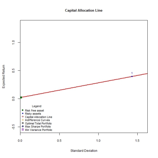
To Implement these functions,let’s first simulate the data for one asset with100 timeseries observations drawn from a normal distribution with a mean and standard deviation that are themselves drawn from a uniform distribution. A risk free rate is also pre-specified at 0.02 and a simple CAL is drawn to connect these 2 assets as per the expression above.

#Capital Allocation Line

sim.one <- simulate.assets(1)
cal.one <-CAL.line('Assets',sim.one,NULL)
DrawCAL(cal.one,sim.one,NULL,legend.draw=TRUE)

As mentioned above, the CAL is simply the combination of the risk free asset and the risky portfolio (which as of yet has been constrained to contain a single asset). The slope of the CAL is the Sharpe ratio and depicts the amount of excess portfolio return per unit of portfolio risk we can expect. Since every point on the CAL is an investment possibility of allocating wealth between the riskless asset and the risky portfolio (single asset in this case), what determines which of these combinations is optimal? The amount of capital an investor places in the risk free asset versus the risky portfolio is determined by the preferences for risk and return as captured by the utility function examined previously.

Mathematically, the objective of an investor is to find the weights of the risky portfolio that maximises the utility of portfolio returns. Or more succinctly :

The optimal weight for the risky portfolio is given by :

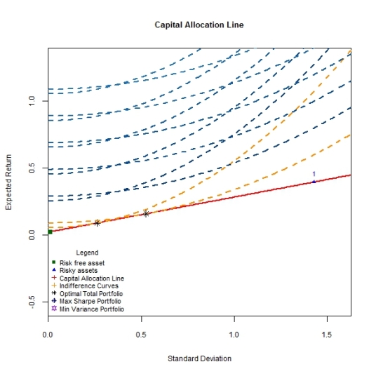
The optimal weight in the risk free asset is then simply (1-w*). Since the indifference curve and the CAL are drawn in the same risk/return space, let’s superimpose an indifference curve with a risk aversion parameter of 1 on the CAL as follows.

utility.contours('Assets',sim.one,1,NULL)

The total optimal portfolio results where investment opportunities as represented by the CAL meet the highest attainable indifference curve as represented by the orange contour. With a risk aversion parameter of 1, the investor exhibits his distaste for risk and places a large weight on the risk free asset versus the risky asset or portfolio. Another investor who is less risk averse (a risk aversion parameter of 0.5) would invest a larger portion of his capital in the risky asset versus the risk free asset and hence the total optimal portfolio is located closer to the simulated risky asset as below.

While the investor prefers to make investments consistent with the risk/return opportunities towards the northwestern corner of the plot – where blue indifference contours are drawn – the available investments as per the capital allocation line do not permit this.

So far we have constrained our risky portfolio to contain only one asset. There is nothing stopping us from simulating multiple risky assets and drawing the CAL between the risk free asset and each of these simulated assets as below.

sim.mult <- simulate.assets(20)
cal.mult <- CAL.line('Assets',sim.mult,NULL)
DrawCAL(cal.mult,sim.mult,NULL,legend.draw=T)

This post has dealt with the second half of the two fund theorem according to which any investment problem can be addressed by combining the risk free asset (riskless fund) and the risky portfolio (risky fund). So far we have constrained the number of assets contained in the risky portfolio. The task of finding the optimal risky portfolio, the second half of the theorem, shall be addressed in the next post.

Asset Pricing [Part 2a : Sketching The Traditional Framework]

Up until the proliferation of the mean-variance analysis due to Markowitz, the typical advice offered by an investment advisor would entail some combination of the following ideas:

• Young investors should allocate a disproportionately large amount of their investable capital to risky securities within risky asset classes.

• Older investors should allocate a disproportionate amount of capital to less volatile securities within less risky asset classes.  

While intuitively compelling and perhaps sensible as a first approximation, linking an individual’s asset allocation decision exclusively to his human capital in such a broad fashion is suboptimal. According to the Two-fund separation theory, a key result in Modern Portfolio Theory, the investment allocation problem can be decomposed into two elements :

(1.) Finding the optimal portfolio of risky assets.

• This amounts to finding a vector of weights associated with risky assets that maximise the risk adjusted return of the resulting portfolio. An important consideration here is the selection and use of an appropriate risk-adjusted performance measure.

(2.) Finding the best combination of the risk free asset and the optimal risky portfolio.

• Once the optimal risky portfolio has been determined, it can be combined with the risk free asset; with respective weights in each of these ‘funds’ subject to individual risk preferences, the total portfolio can be constructed.

The most important implications of Modern Portfolio Theory can be summarised as follows.

• Investors should control total portfolio risk by varying the amount of capital invested in the risk free asset and the optimal risky portfolio as opposed to changing the composition of the risky portfolio itself. The weight given to the either ‘fund’ depends on the individual’s risk aversion.

• The portfolio of risky assets should contain a large number of assets that are less than perfectly positively correlated (i.e. a well diversified portfolio)

It should be noted that most of the relevant results are derived under the assumptions that either [a] all returns are normally distributed or [b] investors care only about mean returns and variance of returns. Further assumptions require that all assets be tradable and no transaction costs are incurred when trades occur.

Before the Two fund theorem can be implemented, a theoretical framework for understanding the tradeoff between risk and return will be briefly sketched.

j

[Utility Functions and Indifference curves]

l

The standard utility function of choice  is the power utility function, also known as constant relative risk aversion or the CRRA utility function.

Gamma, or the coefficient of risk aversion governs the curvature of the utility function and how resistant individuals are to taking risks. It can be shown that the utility an investor derives from a pattern of returns amounts to 

with A representing the risk aversion parameter. If assets can be thought of as providing a benefit (returns) at a cost (risk), then a simple way to visualise the tradeoff can be attained using Indifference curves. To illustrate these and other issues of this post, the following two helper functions,utility.contours and contours.plot were written.

#############################################################################
#
# Contour Plotting
#
#############################################################################

contours.plot <- function(type,expected.ret,risky.var,num.assets,risk.free,risk.aversion,total.risk){

	opt.risky.alloc <- (expected.ret-risk.free)/(risk.aversion* risky.var)
	opt.riskfree.alloc <- (1-opt.risky.alloc)
	opt.port.ret <- risk.free+opt.risky.alloc*(expected.ret-risk.free)
	opt.port.risk <- (opt.risky.alloc^2)*risky.var
	opt.utility <- opt.port.ret-(0.5*risk.aversion*opt.port.risk)

	contours <- vector('list',num.assets)
	  for(i in 1:num.assets){
	  		contours[[i]]$optimal.utility <- opt.utility[i]
	  		contours[[i]]$returns <- opt.utility[i]+(0.5*risk.aversion*total.risk)
	  		contours[[i]]$risk <- sqrt(total.risk)
	  }

	 s.contours <- vector('list',5)
	 u.contours <- vector('list',5)

	  for(i in 1:5){
	      s.contours[[i]]$optimal.utility <- opt.utility[1]
	  		s.contours[[i]]$returns <- opt.utility[1]+(0.5*i*total.risk)
	    	s.contours[[i]]$risk <- sqrt(total.risk)
	  		u.contours[[i]]$optimal.utility <- i
	  		u.contours[[i]]$returns <- opt.utility[1]+i/5+(0.5*risk.aversion*total.risk)
	    	u.contours[[i]]$risk <- sqrt(total.risk)
	  }

	col.indiff <- colorRampPalette(brewer.pal(9,"Blues"))(100)
    ind <- 100

	 if(type=='Sample'){
	  windows()

	  par(mfrow=c(2,1),mar=c(1.5,4,3,1.5))
		plot(main='Indifference Curves',cex.main=0.85,cex.lab=0.75,cex.axis=0.75,ylab='Expected Return',xlab='Risk',x=s.contours[[1]]$risk,y=s.contours[[1]]$returns,type='line',col=col.indiff[ind],lty=2,lwd=2)

	  for(i in 2:5){
      		lines(main='Indifference Curves',cex.main=0.85,cex.lab=0.75,cex.axis=0.75,ylab='Expected Return',xlab='Risk',x=s.contours[[i]]$risk,y=s.contours[[i]]$returns,type='line',col=col.indiff[ind-i*5],lty=2,lwd=2)
    }
 	  legend(title='Utility constant',y.intersp=0.8,adj=0,'bottomright',horiz=F,fill=c(col.indiff[ind],col.indiff[ind-2*5],col.indiff[ind-3*5],col.indiff[ind-4*5],col.indiff[ind-5*5]),legend=c(paste('Risk Aversion: ',1:5)),ncol=1,bg='white',bty='n',border='black',cex=0.70)

		par(mar=c(4,4,1,1.5))
		plot(cex.main=0.85,cex.lab=0.75,cex.axis=0.75,ylab='Expected Return',xlab='Risk',x=u.contours[[1]]$risk,y=u.contours[[1]]$returns,type='line',col=col.indiff[ind],lty=2,lwd=2)

	  for(i in 2:5){
     			lines(main='Indifference Curves',cex.main=0.85,cex.lab=0.75,cex.axis=0.75,ylab='Expected Return',xlab='Risk',x=u.contours[[i]]$risk,y=u.contours[[i]]$returns,type='line',col=col.indiff[ind-i*5],lty=2,lwd=2)
    }
		legend(title='Risk aversion constant',y.intersp=0.8,adj=0,'bottomright',horiz=F,fill=c(col.indiff[ind],col.indiff[ind-2*5],col.indiff[ind-3*5],col.indiff[ind-4*5],col.indiff[ind-5*5]),legend=c(paste('Utility: ',1:5)),ncol=1,bg='white',bty='n',border='black',cex=0.70)

	} else if(type=='Optimal'){

	 lines(cex.main=0.85,cex.lab=0.75,cex.axis=0.75,ylab='Expected Return',xlab='Risk',x=contours[[1]]$risk,y=contours[[1]]$returns,type='line',col='dark orange',lty=2,lwd=2)
	 points(x=sqrt(opt.port.risk),opt.port.ret,pch=8,col='black')

	  for(i in 1:5){
    	lines(x=u.contours[[i]]$risk,y=u.contours[[i]]$returns,type='line',col=col.indiff[ind-i*5],lty=2,lwd=2)
      }
   }
}

##############################################################################
#
# Utility Contours
#
#############################################################################

utility.contours <- function(type,risky.assets,risk.aversion,optimised.portfolio){

	risk.free <- risky.assets[[4]]
	total.risk <- seq(0,2,by=0.01)^2

	if(type=='Assets'){
	  	expected.ret <- risky.assets[[5]]
	  	risky.var <- risky.assets[[3]]^2
	  	num.assets <- length(risky.var)
		contours.plot(type='Optimal',expected.ret,risky.var,num.assets,risk.free,risk.aversion,total.risk)

	 } else if(type=='Sharpe'){
	 	expected.ret <- optimised.portfolio[[4]][1]
	    risky.var <- (optimised.portfolio[[4]][2])^2
	  	num.assets <- 1
	  	contours.plot(type='Optimal',expected.ret,risky.var,num.assets,risk.free,risk.aversion,total.risk)

	 } else if(type=='Indifference Sample'){
	    sim <- simulate.assets(1)
	  	expected.ret <- sim[[5]]
	  	risky.var <- sim[[3]]^2
	  	risk.free.smpl <- sim[[4]]
	  	num.assets <- 1
	  	risk.aversion.smpl <- 1
	  	contours.plot(type='Sample',expected.ret,risky.var,num.assets,risk.free.smpl,risk.aversion.smpl,total.risk)

     } else	if(type=='CRRA'){
		consumption <- seq(0,3,by=0.01)
		gamma <- c(0.7,0.5,0.2)
		util <- matrix(nrow=length(consumption),ncol=length(gamma),c(rep(0,length(consumption)*length(gamma))),byrow=FALSE)
		marginal.util <- matrix(nrow=length(consumption),ncol=length(gamma),c(rep(0,length(consumption)*length(gamma))),byrow=FALSE)

	for(i in 1:length(gamma)){
		util[,i] <- (consumption^(1-gamma[i]))/(1-gamma[i])
		marginal.util[,i] <- consumption^(-gamma[i])
	}

	colnames(util) <- paste('Gamma',1:length(gamma))
	colnames(marginal.util) <- paste ('Gamma',1:length(gamma))
	colours <- colorRampPalette(brewer.pal(9,"Blues"))(100)
	col.index <- 100

	windows()
	 par(mfrow=c(2,1),mar=c(2,2,3,2))
	 plot(cex.axis=0.75,lwd=2,x=consumption,util[,1],type='line',col=colours[col.index],main='Constant Relative Risk Aversion - Utility function',cex.main=0.85,cex.lab=0.75,ylab='')
	 for(i in 2:length(gamma)){
		lines(lwd=3,x=consumption,util[,i],col=colours[col.index-(i*10)])
	 }

	 par(mar=c(3,2,1,2))
	 plot(cex.axis=0.75,ylim=c(-3,3),lwd=2,x=consumption,marginal.util[,1],type='line',col=colours[col.index],main='Constant Relative Risk Aversion - Marginal Utility function',cex.main=0.85,cex.lab=0.75,ylab='')
	 for(i in 2:length(gamma)){
		lines(lwd=2,x=consumption,marginal.util[,i],col=colours[col.index-(i*10)])
	 }
	 legend(horiz=TRUE,title='Gamma',"bottom",fill=c(colours[col.index],colours[col.index-20],colours[col.index-30]),legend=gamma[1:3],bg='white',bty='n',border='white',cex=0.75)
   }
}

To Implement these functions :

##############################################################
#
# Implementations
#
##############################################################

#Utility Contours

utility.contours(type='CRRA',risky.assets=NULL,risk.aversion=NULL,optimised.portfolio=NULL)
utility.contours(type='Indifference Sample',risky.assets=NULL,risk.aversion=0.5,optimised.portfolio=NULL)

The plots above illustrate the CRRA utility function as well as its first derivative (or marginal utility function). The greater the risk aversion coefficient ,gamma, the greater the curvature of the utility function, the more risk averse an individual, the larger the amount of money (the certainty equivalent) required to make that individual indifferent between receiving a particular money amount with perfect certainty and obtaining that amount as an expectation of a gamble. The slope of the utility curve,as depicted in the bottom plot as the first derivative of the preceding function , suggests that the additional utility derived from an extra unit of wealth declines as the amount or level of wealth increases. While utility derived increases with wealth, the rate at which an additional unit of wealth promotes greater utility decreases over rising wealth.

The first plot depicts the effect on indifference curves of varying the risk aversion parameter while holding utility constant. The converse is true for the second plot, in which the risk aversion parameter is held constant across varying degrees of utility while indifference curves are charted. True to its name, an indifference curve connects all combinations of (in this case) risk and return which yield the same utility. With respect to the first plot, the greater the risk aversion of an individual, the greater the expected return required for a given level of risk before the specified level of utility can be reached. With respect to the second plot, northwesterly movements of the contour signify combinations of risk and return that yield greater utility. Intuitively, when risk aversion and risk are held constant, the asset that provides greater expected returns would command greater utility. An investor, who regards assets as bundles of risks and returns, would wish to hold a portfolio of assets that are located on the highest possible indifference curve for a given aversion to risk.