Asset Pricing [8c : Time Series Predictability]

The point of the Campbell-Shiller present value identity is to quantitatively illustrate how variance in dividend yields must be matched by the variable’s ability to forecast returns and/or dividend growth.

The price-dividend ratio can move if and only if there is corresponding news about current dividends,future dividend growth or future returns. If returns and dividend growth are totally unpredictable (i.e. if at every time (t), a trader’s expectation of future dividend growth and returns are constant), then p(t)-d(t) must be constant. Since dividend yields are demonstrably varying over time, asset markets cannot feature both unpredictable dividends and unpredictable returns.

The previous post examined how the introduction of new variables (dividend yield) and long horizon regressions (k=1:15) overturned previously cherished beliefs about the unpredictability of returns. While the results can be (and were) framed in the context of the Campbell-Shiller identity, we have not really tested the identity’s implications empirically.We have neither run infinite order regressions on log variables :

nor determined that the long-run return and dividend growth regression coefficients mechanically add up to one :

I have merely shown how returns (which should be unpredictable) are increasingly forecastable at longer horizons on the basis of the dividend yield, and how dividend growth (which should be forecastable) eludes forecastability at any horizon by the same measure. In the following code snippet I have transformed the raw variables into logs, compounded the return and dividend growth variables across a finite horizon (1:15 as before) before using them as inputs to the set of long-run regressions. Since one cannot actually run infinitely long regressions,I used the VAR’s implications for infinite period forecasts to determine the long-run coefficient of the return regression :

 

The code follows :

#####################################################################################
# Long-run forecasts using Campbell Shiller identity
#####################################################################################

idx.list dg.list idx.reg dg.reg
idx.list[[1]] dg.list[[1]] <-log.dg

for(i in 2:15){
 idx.list[[i]]=LogCompound(log.ret,i)
 dg.list[[i]]=LogCompound(log.dg,i)
}

for(i in 1:15){
  temp=cbind(idx.list[[i]],lag(log.dp,-1)[1:length(idx.list[[i]])])
  temp2=cbind(dg.list[[i]],lag(log.dp,-1)[1:length(dg.list[[i]])])
  idx.reg[[i]]=lm(temp[,1]~temp[,2])
  dg.reg[[i]]=lm(temp2[,1]~temp2[,2])
}

idx.coef=sapply(idx.reg,coef)[2,]
dg.coef=sapply(dg.reg,coef)[2,]
coef.diff=idx.coef-dg.coef

#Infinite order
temp3=cbind(log.dp,lag(log.dp,-1),log.ret)
dp.coef=coef(lm(temp3[,1]~temp3[,2]))[2]
temp4=cbind(log.ret,lag(log.dp,-1))
ret.coef=coef(lm(temp4[,1]~temp4[,2]))[2]
infinite.br=(1/rho)*(ret.coef/(1-(rho*dp.coef)))
infinite.dg=infinite.br-1

b.data=rbind(idx.coef,dg.coef)
lr.data=cbind(matrix(0,nrow=2,ncol=15),c(infinite.br,infinite.dg))
lr.df=cbind(matrix(0,nrow=1,ncol=15),(infinite.br-infinite.dg))

windows()
b=barplot(ylim=c(0,max(lr.data)+0.5),axes=F,xlab='Horizon',b.data,cex.main=0.85,cex.lab=0.75,cex.axis=0.75,main='Long-run coefficients and their differences\nacross horizons',col=c('darkblue','lightblue'))
barplot(coef.diff,col='cyan',add=T,axes=F)
barplot(lr.df,col='gold',add=T,names.arg=c(1:15,expression(infinity)))
text(b,coef.diff-0.05,round(coef.diff,2),cex=0.7,col='black')
text(b[15]+(b[15]-b[14]),lr.df[16]-0.05,round(lr.df[16],2),cex=0.7,col='black')
text(1.5,1.05,'1~b(r)-b(dg)',col='red',cex=0.7,font=2)
legend(bty='n',y.intersp=0.85,'left',fill=c('darkblue','lightblue','cyan','gold'),legend=c('long-run b(r)','long-run b(dg)','difference(horizons)','difference(infinite order VAR)'),ncol=1,bg='white',cex=0.7)
###################################################################################

kk
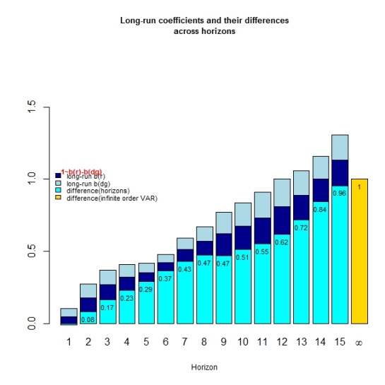
This produces a barchart which shows how the long run return and dividend growth coefficients as (well as their differences) vary across forecast horizons (both finite and infinite).

Clearly,longer forecast horizons increasingly satisfy the mechanical requirement of long run coefficients summing to one.We have started with the observation that variance in dividend yields must be matched by the variable’s ability to forecast returns and/or dividend growth. Now we have empirically determined which of these two possible channels is responsible for the observed variation in the price ratio : time-varying discount rates explain virtually all the variance of market dividend yields whereas dividend growth forecasts explain essentially none if it. In other words,variation in dividend yield corresponds completely to expected return news rather than to cashflow news. Expected return is the dominant cause of market price movements.

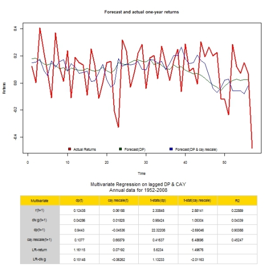
While I have focussed on D/P regressions so far, there are evidently a host of other variables that help forecast returns. Among these,Lettau & Ludwigson’s consumption-to-wealth ratio (cay) makes for an interesting candidate since it affects the term structure of expected returns in a way that is useful in the short run and that can be beautifully captured using impulse response functions. Consider the usual set of forecasting regressions with dp(t) and an additional cay(t) as state variables for both the single period and multi-period (long horizon) case. I have arbitrarily set the long horizon to k=15 for this example.An infinite order VAR would have been more appropriate but I do not know how to compute the implications for long-run coefficients in the case of multiple variables. Before using the cay variable in the regression,I rescaled it to have a standard deviation of 1 (as was done in the lecture).

k

###################################################################################
# Forecasting regressions with CAY variable
###################################################################################

cay.rescale=(cay/sd(cay))
reg.list <- list()
temp <- cbind(log.ret,log.dg,log.dp,cay.rescale,lag(log.dp,-1),lag(cay.rescale,-1))
temp2<-cbind(log.ret,lag(log.dp,-1))
dp.reg=lm(temp2[,1]~temp2[,2])

#One period regression
for(i in 1:4){
  reg.list[[i]]=lm(temp[,i]~temp[,5]+temp[,6])
}

#Long-run regressions
data1=cbind(idx.list[[15]],lag(log.dp,-1)[1:length(idx.list[[15]])],lag(cay.rescale,-1)[1:length(idx.list[[15]])])
lrun.ret.reg=lm(data1[,1]~data1[,2]+data1[,3])

data2=cbind(dg.list[[15]],lag(log.dp,-1)[1:length(dg.list[[15]])],lag(cay.rescale,-1)[1:length(dg.list[[15]])])
lrun.dg.reg=lm(data2[,1]~data2[,2]+data2[,3])

#Extracting estimates
estim=rbind(RegExtractor(reg.list,'est')[,-1],coef(lrun.ret.reg)[-1],coef(lrun.dg.reg)[-1])
tvals=rbind(RegExtractor(reg.list,'tval')[,-1],coef(summary(lrun.ret.reg))[c(2:3),3],coef(summary(lrun.dg.reg))[c(2:3),3])
rsq=matrix(RegExtractor(reg.list,'rsq'),ncol=1)

#Plot & Table
row.names<- c('r(t+1)','div.g(t+1)','dp(t+1)','cay.rescale(t+1)','LR-return','LR-div.g')
col.names<-c('dp(t)','cay.rescale(t) ','t-stats(dp)','t-stat(cay.rescale)','R2')
reg.table=cbind(round(estim,5),round(tvals,5),rbind(round(rsq,5),' ',' '))

windows()
layout(matrix(c(1,1,2),nrow=3))
plot(x=1:57,y=lag(log.ret,+1),ylab='Returns',xlab='Time',cex.main=0.85,cex.lab=0.75,cex.axis=0.75,main='Forecast and actual one-year returns',col='red',type='l',lwd=2)
lines(fitted(dp.reg),col='darkgreen',lwd=1)
lines(fitted(reg.list[[1]]),col='blue',lwd=1)
legend(bty='n',y.intersp=1,'bottom',fill=c('red','darkgreen','blue'),legend=c('Actual Returns','Forecast(DP)','Forecast(DP & cay.rescale)'),ncol=3,bg='white',cex=0.75)

est.tab <- reg.table
est.tab <- apply(est.tab, 2, rev)
est.tab <- cbind(rev(row.names),est.tab)
par(mai=c(0.15,0.25,0.25,0.15))
		TableMaker(row.h=1,est.tab,c('Multivariate',col.names),strip=F,strip.col=c('green','blue'),col.cut=0.05,alpha=0.7,border.col='lightgrey',text.col='black',header.bcol='gold',header.tcol='black',title=c('Multivariate Regression on lagged DP & CAY\nAnnual data for 1952-2008'))
###################################################################################

kThe figure above graphs the one year forecast using [1] the dividend yield alone and [2] both dividend yield and consumption-to-wealth ratio against actual ex-post returns. Clearly, adding the cay variable allows us to capture the undulations of actual returns that would have otherwise gone unnoticed.The first four rows of the accompanying table show regression results for one year estimates while the last two rows show the results for long horizon regressions. In the short run, the cay variable helps to forecast one-period returns.The t-statistic is relatively large and the R-squared of 23% implies that the variation of expected returns is substantially raised.The new variable only marginally helps to forecast dividend growth. The cay signal decays more quickly than dp,with a 0.66 coefficient as opposed to 0.94. From these one-period results it is tempting to conclude that we have found a potent new forecaster in the cay variable. These rosy results however are overturned in the long run where the cay coefficient becomes statistically indistinguishable from 0. Even though the consumption-to-wealth ratio has a dramatic effect on one-period return forecasts ,it has almost no effect on long-run return forecasts. It is in this sense that the new variable affects the term structure of expected returns.

• campbell shiller
• infinite order VAR
• R