Asset Pricing [7a : Macroeconomic factor model]
The ability of investors to manage a portfolio of assets that are less than perfectly correlated with one another – thus conferring diversification benefits to total investment risks for a given level of portfolio return – is consistent with the focus of modern financial theory in seeking out pervasive (systematic) influences as the likely source of priced undiversifiable risk. The general conclusion of theory is that capital markets should only award investors with an additional return component if they are exposed to a set of risk factors whose influence on total risk cannot be mitigated by holding a diversified set of assets. On balance, the stridency with which financial theories expound their conclusions is only matched by their relative timidity in terms of identifying the exogenous influences,the economic state variables that underlie comovements of asset prices. The objective of this post is to apply a simplified version of the Chen,Roll&Ross (1986) methodology (effectively a Fama MacBeth procedure) to a random sample of 25 stocks on the SP500 index. The authors begin by identifying macroeconomic variables that should systematically affect stock returns and proceed to test whether surprises (innovations) in these factors represent risks that are rewarded by the market.
To ascertain whether the identified economic state variables are related to the underlying factors that explain asset pricing,a version of the Fama-MacBeth methodology shall be employed.
[The model and its data]
The macroeconomic factor model is specified as follows :
![]() with independent variables on the right hand side being factor surprises or innovations defined according to
with independent variables on the right hand side being factor surprises or innovations defined according to
and f being macroeconomic variables of interest. According to the original authors, the following economic variables should systematically affect stock returns : [1] Spread between long/short rates , [2] Change in expected Inflation , [3] Unexpected Inflation , [4] Industrial Production , [5] Spread between high and low grade bonds.
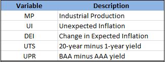
While I have neither access to databases that contain these datasets nor patience to scrape individual variables separately from the web (if that is even possible), I do have access to Google and the requisite patience to find entire data sets (usually) provided by university professors on their course websites. This time it is from Hong Kong of all places. I have summarised the variable names used throughout the code for convenience :
In terms of test assets used on the left hand side, i simply took a random sample of 25 stocks from the SP500 index and compute their returns. I have previously saved price/return data for stocks on the SP500 in an RData file,hence I shall simply take my sample from there instead of downloading new data.
[Estimation procedure – Fama/MacBeth]
[1] Time series regression of stock returns on unanticipated changes in macroeconomic variables to yield asset exposures to risk factors.
[2] In each month, a cross section regression of stock returns on previously estimated asset exposures to a time series of risk premia and pricing errors.
[3] Take mean of these time series and test for significance.
[4] Joint Test
with
The above procedure can be replicated for rolling windows as well, in which case 5 years worth of data are used in the initial time series regression and the cross section regressions are applied to each of the 12 months in the subsequent year before the window of fixed size is rolled forward and the process repeated. As with all posts on this blog, these are mere experiments, very likely erroneous in some way and not meant for replication.

