Asset Pricing [8f : Replicating Cochrane’s Dog 2]

The previous post outlined the dataset,custom functions used throughout the code as well as some of the intuition behind Cochrane’s(2008) paper. Now we shall continue with the actual implementation of the simulation procedures and steps previously listed.

[1] Obtain original sample estimates (1927-2004) and the error covariance matrix by running the three VAR regressions. This step provides the inputs needed for the subsequent simulation.

After subsetting our original dataset to contain only data for the 1927-2004 date range across transformed variables, I ran the following single period forecasting regressions :

Lowercase variables denote log-transformed variables as usual.The last three equations are the familiar VAR regressions mentioned in previous posts and provide the inputs necessary for the simulation. The first three regressions are just there for completeness sake (they are run by Cochrane as well).These set of equations basically replicate some of the information contained in Tables 1&2 of the paper albeit without inflation adjustments. In the following code, I :

• stored each of the above regressions as an element of a list object.
• The custom RegExtractor)() function is then called to extract regression summaries from this list object using the sapply() function.
• The output is then tabulated using the TableMaker() function.

 

######################################################################################
# Initial single period regression
######################################################################################

#Single Period regressions
initial.reg <- list(
	ret_divyield=dyn$lm(Idx.ret~lag(Div.yield,-1),data=orig.extract),
	exret_divyield=dyn$lm(Exc.ret~lag(Div.yield,-1),data=orig.extract),
	dgrowth_divyield=dyn$lm(Div.growth~lag(Div.yield,-1),data=orig.extract),
	log_ret_divyield=dyn$lm(log.ret~lag(log.div.yield,-1),data=orig.extract),
	log_divgrowth_divyield=dyn$lm(log.div.growth~lag(log.div.yield,-1),data=orig.extract),
	log_divyield_divyield=dyn$lm(log.div.yield~lag(log.div.yield,-1),data=orig.extract)
)
reg.names <- names(initial.reg)

#Extract regression values
betas <- matrix(RegExtractor(initial.reg,'est')[,2],ncol=1)
tvals <- matrix(RegExtractor(initial.reg,'tval')[,2],ncol=1)
pvals <- matrix(RegExtractor(initial.reg,'pval')[,2],ncol=1)
rsq <- matrix(RegExtractor(initial.reg,'rsq'),ncol=1)*100
res <- matrix(RegExtractor(initial.reg,'res'),ncol=6,dimnames=list(NULL,reg.names))
res.cov <- cbind(res[,'log_divgrowth_divyield'],res[,'log_divyield_divyield'])
std.vals <- sapply(initial.reg,function(v) sd(fitted(v)))*100

#Table
col.names <- c('Beta','t-stats','p-vals','R2','Std(Fitted)')
reg.table = cbind(betas,tvals,pvals,rsq,std.vals)

est.tab <- round(reg.table,5)
est.tab <- apply(est.tab, 2, rev)
est.tab <- cbind(rev(reg.names),est.tab)
TableMaker(row.h=1,est.tab,c('Single Period',col.names),strip=F,strip.col=c('green','blue'),col.cut=0.05,alpha=0.7,border.col='lightgrey',text.col='black',header.bcol='gold',header.tcol='black',title=c('Regression on lagged variables\nAnnual data for 1926-2004'))

gg

This results in the following :

The inputs used in the Null hypothesis are

• b(r)=0 and phi=0.94125.The value for phi is simply the coefficient estimate of the log_divyield_divyield regression (last row of table).
• ρ=0.9638 (from the Cochrane paper)
• the dividend forecast coefficient follows from the identity as b(d) = ρφ − 1 + b(r)≈ −0.1
• sample estimates of the covariance matrix from div_growth and div_yield regression.

Such that the Null takes the form of :

 

---

[2 & 3] Each of the 20000 monte carlo trials (50000 in the paper) generates a dataset.Once we have 20000 simulated datasets,we run each of the VAR regressions for each simulated dataset and collect regression estimates.

From the paper : I simulate 20,000 artificial data sets from each null. For φ < 1, I draw the first observation d0 − p0 from the unconditional density d0 − p0 ∼ N(0, σ2(εdp)/(1 − φ^2).For φ ≥ 1, I start at d0 − p0 = 0. I,then draw εdt
and εdpt as random normals and simulate the system forward.

• inputs from the previous step are fed into the MonteCarloSimulation() function which calls the SimulateVAR function() to generate and return the simulated data.
• with each simulated dataset,the MonteCarloSimulation() function continues with our conventional VAR regressions.
• such that for each trial of the simulation we calculate and store the following : b(r),b(d),phi,t-stats for each variable,b(long.r),b(long.d)
• ultimately,the MonteCarloSimulation() function returns a list object with 2 elements.
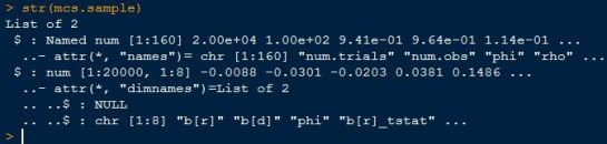
• the first element is a summary of the inputs used/provided by the user
• the second element of that list contains the simulated results with rows representing trials, and columns representing different stats (e.g. coefficients,tstats)

 

In terms of the code, I have made it such that I only run the simulation once for the sample and once for the fixed case of phi=0.99 (as Cochrane does this too) and save those results, along with the sample regressions and their stats (from step 1), in an RData file.

 

# Run Montecarlo simulation
mcs.sample <- MonteCarloSimulation(num.trials=20000,num.obs=100,phi=betas[6],rho=0.9638,error.cov=res.cov)
mcs.fixed <- MonteCarloSimulation(num.trials=20000,num.obs=100,phi=0.99,rho=0.9638,error.cov=res.cov)

#Save all the sample estimates,and simulation results in a .Rdata file
save(initial.reg,betas,tvals,pvals,rsq,res.cov,mcs.sample,mcs.fixed,file='DogBark.Rdata')

ll

By saving the simulation results we are also saving time.Loading the data back into R is as simple as :

 

#Load data
load('DogBark.Rdata')

lll

So far we have run all the regressions and simulations intended and saved the resulting sample and simulation data in a convenient .RData file for simple access. The next post will examine the marginal and joint distributions of simulated parameter estimates,their respective test statistics as well as long horizon issues and the effects of varying phi on estimates.

• cochrane
• Joint Distribution plots
• R
• simulation
• VAR regressions