Archive

Tag Archives: DEA

In the previous post we visualised the quarterly returns for the 30 components of the DJIA between 2005-2009. After ranking quarterly performance of each stock , we proceeded to regress excess monthly log returns on the Fama & French factors in both the standard OLS and the more robust QRS frameworks. This post will focus on applying an input- oriented -variable- returns- to- scale DEA model to requisite inputs and outputs for each stock. While the regression coefficients extracted from the OLS and QRS procedures for each year constitute the inputs to the DEA model, the annualised returns for each stock represent associated outputs for each DMU. Before these attributes can be passed to the DEA model, it is first necessary to standardise and rescale them. The methodology is detailed in the links provided in the previous post.

l

windows()
    par(mai=c(0.1,0.5,0.5,0.5),mfrow=c(6,1))
    barplot(main="DEA applied to Quantile inputs",cex.names=0.9,horiz=F,cex.axis=0.9,beside=F,eff.05[,1],col=ifelse(round(t(eff.05[,1])[1,],2)<1.00,"red","blue"),las=2,xaxt='n')
    mtext(side=4,Years[1],cex=0.7)
    barplot(cex.names=0.9,horiz=F,cex.axis=0.9,beside=F,eff.06[,1],col=ifelse(round(t(eff.06[,1])[1,],2)<1.00,"red","blue"),las=2,xaxt='n')
    mtext(side=4,Years[2],cex=0.7)
    barplot(cex.names=0.9,horiz=F,cex.axis=0.9,beside=F,eff.07[,1],col=ifelse(round(t(eff.07[,1])[1,],2)<1.00,"red","blue"),las=2,xaxt='n')
    mtext(side=4,Years[3],cex=0.7)
    barplot(cex.names=0.9,horiz=F,cex.axis=0.9,beside=F,eff.08[,1],col=ifelse(round(t(eff.08[,1])[1,],2)<1.00,"red","blue"),las=2,xaxt='n')
    mtext(side=4,Years[4],cex=0.7)
    barplot(cex.names=0.9,horiz=F,cex.axis=0.9,beside=F,eff.09[,1],col=ifelse(round(t(eff.09[,1])[1,],2)<1.00,"red","blue"),las=2)
    mtext(side=4,Years[5],cex=0.7)
    plot.new()
    legend("center",title="Data Envelopement Analysis",fill=c("blue","red"),legend=c("Efficient","Inefficient"),ncol=2)

windows()
    par(mai=c(0.1,0.5,0.5,0.5),mfrow=c(6,1))
    barplot(main="DEA applied to OLS inputs",cex.names=0.9,horiz=F,cex.axis=0.9,beside=F,eff.ols.05[,1],col=ifelse(round(t(eff.ols.05[,1])[1,],2)<1.00,"red","blue"),las=2,xaxt='n')
    mtext(side=4,Years[1],cex=0.7)
    barplot(cex.names=0.9,horiz=F,cex.axis=0.9,beside=F,eff.ols.06[,1],col=ifelse(round(t(eff.ols.06[,1])[1,],2)<1.00,"red","blue"),las=2,xaxt='n')
    mtext(side=4,Years[2],cex=0.7)
    barplot(cex.names=0.9,horiz=F,cex.axis=0.9,beside=F,eff.ols.07[,1],col=ifelse(round(t(eff.ols.07[,1])[1,],2)<1.00,"red","blue"),las=2,xaxt='n')
    mtext(side=4,Years[3],cex=0.7)
    barplot(cex.names=0.9,horiz=F,cex.axis=0.9,beside=F,eff.ols.08[,1],col=ifelse(round(t(eff.ols.08[,1])[1,],2)<1.00,"red","blue"),las=2,xaxt='n')
    mtext(side=4,Years[4],cex=0.7)
    barplot(cex.names=0.9,horiz=F,cex.axis=0.9,beside=F,eff.ols.09[,1],col=ifelse(round(t(eff.ols.09[,1])[1,],2)<1.00,"red","blue"),las=2)
    mtext(side=4,Years[5],cex=0.7)
    plot.new()
        legend("center",title="Data Envelopement Analysis",fill=c("blue","red"),legend=c("Efficient","Inefficient"),ncol=2)


c

The collection of bar-plots above summarises the efficiency scores for each asset in each of the 5 years of data. In this case we are using OLS derived Fama and French coefficients as inputs to the DEA model for each stock. While the blue bars correspond to efficient stocks, the red bars represent inefficient DMUs.

o

f

The second collection of bar-plots above summarises the efficiency scores for each asset in each of the 5 years of data. In this case we are using QRS derived Fama and French coefficients as inputs to the DEA model for each stock. While the blue bars correspond to efficient stocks, the red bars represent inefficient DMUs. Now that we have determined the subset of the 30 index components that can be deemed efficient in each year using different inputs, let’s construct equally weighted portfolios of these efficient stocks for each year and input set and compare performance. Based on QRS inputs and DEA results, the portfolio constructed in 2009 for example is equally weighted across AXP,IBM,INTL,JNJ, KFT,MSFT,PFE,PG,UTX.

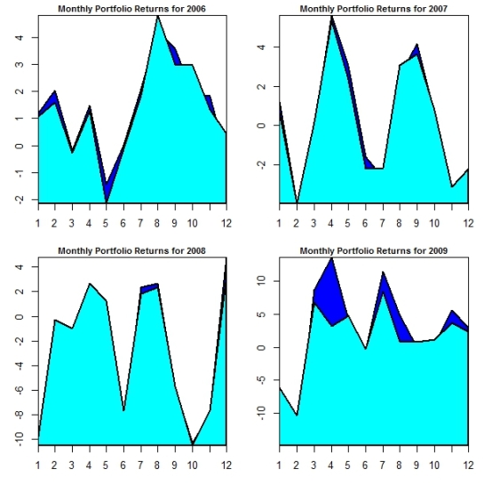
Above is a collection of stacked polygon plots that compares the monthly returns for OLS derived (darkblue) vs QRS derived(cyan) portfolios for 4 years (2006-2009). With the exception of a handful of months in each year, the OLS derived coefficients appear to create superior portfolio returns that the QRS derived counterparts. Only in 2008 , does the QRS portfolio appear to provide some consistency in the benefits of applying a more robust method to the data. As the table below shows,annualising portfolio returns does not seem to help much either. Contrary to expectations the OLS derived portfolio actually is better than the QRS counterpart. The only exception is in 2007-2008 where the QRS portfolio generates less negative returns than the OLS counterpart.

Quantile OLS
2006 15.770552 16.315416
2007 2.443413 3.332335
2008 -31.224554 -35.138542
2009 15.439622 27.783856

f
While the number range is somewhat comparable to those found in the study (link in previous post), we don’t replicate the superiority of QRS portfolios here. The discrepancy is probably due to my mistakes somewhere in the convoluted code. Non the less, it should be noted that the study used the 2005 DJIA components while I used the current index composition. Instead of CISCO and Traveller’s companies, the study had GM and CITI.

In this post the theory of Data Envelopment Analysis (DEA) will be applied to security selection and simple portfolio construction.DEA is used for evaluating and comparing performances of organizational units in a multi-attribute and multidimensional environment by determining the relative efficiency of a decision-making-unit (DMU). More precisely, if one can define stocks as individual decision-making-units (DMU), each associated with single/multiple dimensional inputs and outputs, it should be possible to compute an efficiency score, that encompasses all associated costs and benefits, for each asset. A security is considered efficient if its composite measure of output offsets its corresponding composite measure of input. I suppose in this context, a security can be regarded as efficient if no other combination of costs( inputs) can yield a greater benefit (output). While inputs and outputs associated with each DMU (i.e.asset) can be defined in a number of ways, here we shall use a stock’s Fama & French coefficients as inputs and annualised returns as outputs. More precisely,we shall regress each stock’s monthly excess returns, calculated from log closing prices, on Fama & French’s factor returns using OLS as well as a quantile regression framework. The first link below summarises the methodology used.

Click here for the  complete post ::  Click here for the Fama/French dataset

i

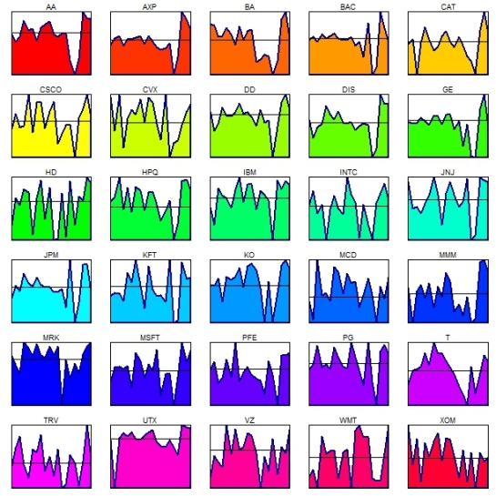
After downloading stock data for the 30 components of the Dow Jones Industrial Average index from 2005 to 2009, let’s first visualise the quarterly returns for each asset and rank the stocks according to their returns.
l

#Visualise Quarterly returns

quarterly.matrix&lt;-assets$quarterly.returns[[1]]
for(i in 2:n.assets){
  quarterly.matrix&lt;-cbind(quarterly.matrix,assets$quarterly.returns[[i]])
}

tq&lt;-t(quarterly.matrix)
colnames(tq)&lt;-rownames(quarterly.matrix)
rm&lt;-rowMeans(tq)

windows()
par(mfrow=c(6,5),mai=c(0.1,0.15,0.15,0.1),xaxt='n')
cb&lt;-rainbow(30)
for(i in 1:30){

  stackpoly(axis2=F,axis4=F,lwd=2,border=&quot;darkblue&quot;,xlab='',cex.axis=0.75,quarterly.matrix[,i],cex.main=0.85,col=cb[i])
  abline(h=0,lwd=1,col=&quot;black&quot;)
  mtext(text=index.comp[i],side=3,col='black',cex=0.6)
}

windows()
par(mfrow=c(2,2),mai=c(0.5,0.5,0.5,0.2))

for(i in 1:4){
  barplot(cex.names=0.67,horiz=T,cex.axis=0.75,beside=FALSE,border='white',tq[order(tq[,i]),][,i],las=2,main=paste(&quot;Best/Worst Performances for Quarter&quot;, i),cex.main=0.85,col=ifelse(tq[order(tq[,i]),][,i]&lt;=0,&quot;red&quot;,&quot;green&quot;))
  abline(v=0,lwd=2,col=&quot;blue&quot;)
  minm&lt;-min(tq[order(tq[,i]),][,i])
  maxm&lt;-max(tq[order(tq[,i]),][,i])
  t&lt;-as.matrix(tq[order(tq[,i]),][,i])
  rmin&lt;-rownames(t)[1]
  rmax&lt;-rownames(t)[30]
  text(x=minm/2,y=30,paste(&quot;min :&quot;,rmin,round(t[1],2)),cex=0.75,col=&quot;red&quot;)
  text(x=minm/2,y=32,paste(&quot;max :&quot;,rmax,round(t[30],2)),cex=0.75,col=&quot;green&quot;)
}

s

Next let’s regress the monthly excess asset returns on Fama-French factor returns using standard OLS as well as the quantile regression framwork for each year in the dataset. Using the rpanel package, we can once again make use of the slider control which allows us to plot the OLS derived coefficients for each designated year.

d

windows()
par(mfrow=c(3,1),mai=c(0.5,0.5,0.5,0.5))
if (interactive()) {
  draw &lt;- function(panel) {
    barplot(space=0.5,cex.names=0.9,horiz=F,cex.axis=0.9,beside=T,tot.mkt[[panel$Year]],las=2,main=paste(&quot;Fama-French Betas for MKT\n&quot;,Years[[panel$Year]]),cex.main=0.95,col=&quot;orange&quot;)
    barplot(space=0.5,cex.names=0.9,horiz=F,cex.axis=0.9,beside=T,tot.smb[[panel$Year]],las=2,main=paste(&quot;Fama-French Betas for SMB\n&quot;,Years[[panel$Year]]),cex.main=0.95,col=&quot;green&quot;)
    barplot(space=0.5,cex.names=0.9,horiz=F,cex.axis=0.9,beside=T,tot.hml[[panel$Year]],las=2,main=paste(&quot;Fama-French Betas for HML\n&quot;,Years[[panel$Year]]),cex.main=0.95,col=&quot;blue&quot;)
    panel
  }
  panel&lt;- rp.control(Year = 1)
  rp.slider(panel,Year, 1,5, action=draw,resolution=1,showvalue=TRUE

s

k

Unfortunately, 3d-surface plots cannot be that easily updated using the slider function, limiting the surface plots to one asset at a time. The first is a surface plot of factor returns across quantiles which probably does not make much sense but looks pretty non the less. The next 3 plots show how the MKT,SMB,HML coefficients (as per Fama and French) vary across quantiles and time. From these plots it is evident that high/med/low return stocks respond very differently to risk factors across time.

l

md&lt;-expand.grid(MKT=MKT.tot$asset[[1]],SMB=SMB.tot$asset[[1]])
mm&lt;-expand.grid(Quantiles=Quantiles,Years=Years)
dataf&lt;-data.frame(MKT=md$MKT,SMB=md$SMB,HML=HML.tot$asset[[1]])
dr&lt;-seq(-2,2,0.1)
l&lt;-length(dr)

windows()
wireframe(useRaster=T,region=T,alpha.regions=0.5,at=dr,col.regions=rainbow(l),main=paste(&quot;Beta Plots for&quot;,index.comp[1]),data=dataf,HML~MKT*SMB,screen = list(z =-15, x =-70),colorkey=TRUE,drape=T)

windows()
dataf2&lt;-data.frame(Quantiles=mm$Quantiles,Years=mm$Years,MKT=MKT.tot$asset[[1]])
wireframe(main=paste(&quot;MKT across quantiles and time for&quot;,index.comp[1]),useRaster=T,region=T,alpha.regions=1,at=c(-2,-1.5,-1,0,1,1.5,2),col.regions=brewer.pal(7,&quot;Blues&quot;),data=dataf2,MKT~Years*Quantiles,screen = list(z =-15, x =-70),colorkey=TRUE,drape=T)

windows()
dataf3&lt;-data.frame(Quantiles=mm$Quantiles,Years=mm$Years,SMB=SMB.tot$asset[[1]])
wireframe(main=paste(&quot;SMB across quantiles and time for&quot;,index.comp[1]),useRaster=T,region=T,alpha.regions=1,at=c(-2,-1.5,-1,0,1,1.5,2),col.regions=brewer.pal(7,&quot;Greens&quot;),data=dataf3,SMB~Years*Quantiles,screen = list(z =-15, x =-70),colorkey=TRUE,drape=T)

windows()
dataf4&lt;-data.frame(Quantiles=mm$Quantiles,Years=mm$Years,HML=HML.tot$asset[[1]])
wireframe(main=paste(&quot;HML across quantiles and time for&quot;,index.comp[1]),useRaster=T,region=T,alpha.regions=1,at=c(-2,-1.5,-1,0,1,1.5,2),col.regions=brewer.pal(7,&quot;Reds&quot;),data=dataf4,HML~Years*Quantiles,screen = list(z =-15, x =-70),colorkey=TRUE,drape=T)

d