Archive

Tag Archives: Capital asset pricing model

The Fama-French 3 factor model is an extension of the market model to the tune of two additional factors to explain security/portfolio returns : the size premium and the book-to-market (value) premium. The model was developed in response to prior research and empirical observations that indicated systematic outperformance of small firm / value stocks versus large firm / growth stocks and the market as a whole. From the previous post it is clear that variation in size produces a variation in average returns that is positively related to variation in market betas, the central risk-return relation posited by the CAPM. By contrast,variation in the book-to-market ratio produces a variation in average returns that is negatively aligned to variation in market betas,violating the central implication of risk-return models.

The Carhart 4 factor model extends the FF3F model with the addition of a momentum factor. The inclusion of this fourth factor is a response to studies that showed how stocks with strong past performance continue to outperform stocks with poor performance in the next period gathering an average excess return of 1% per month (Jegadeesh & Titman,1993)

In some sense, the FF3F model is a synthesis of a string of anomalies that contradict CAPM predictions. The literature surrounding CAPM implications (and more importantly their contradictions) focuses on sorting stocks according to some characteristic (size,value,financial ratios), relating this sorted set of assets with their average returns and econometrically aligning them to market risk. To put the findings in context, the following summarises one of the many literature surveys easily found on the internet.

g

[Survey of contradictions]

:: Earnings/Price Ratio

The earliest blow to the CAPM came from Basu(1977) who showed that stocks with high E/P ratios earned significantly higher returns than assets with low E/P ratios. Since differences in beta could not explain these return differences,the E/P effect is a direct contradiction of the CAPM.

:: Firm Size

The size effect,uncovered by Banz(1981),indicates that stocks of firms with low market capitalisations have higher average returns than large cap stocks. While smaller firms also suffer from greater market risk and hence preserve a positive risk-return relation required by theory, the beta differences are unfortunately not large enough to explain the observed return differences to conform to CAPM predictions.

:: Long-Term Return Reversals

Defining ‘losers’ as stocks that have had poor returns over the past 3-5 years and ‘winners’ as those stocks that had high returns over a similar period,Debondt and Thaler(1985) found that losers tend to have much higher average returns than winners over the next 3 to 5 years. The key question,of whether or not the superior returns associated with looser stocks are aligned with higher systematic risk, had been settled in the early 1990s by Lakonishok and Ritter (1992) who suggested that the variation in beta cannot account for this difference in average returns between losers and winners.

:: Book-to-Market Ratio

Rosenberg,Reid and Lanstein(1985) found that stocks with high book-to-market ratios have significantly higher returns than stocks with lower values for this ratio. This variable still produces significant dispersion in average returns that cannot be explained with the CAPM alone.

:: Leverage

Bhandri(1988) found that firms with high leverage (measured by the debt/equity ratio) have higher average returns than firms with less debt even after controlling for size and market beta. The increased riskiness of a highly leveraged firm’s equity should be reflected in a higher beta coefficient.

:: Momentum

Jegadeesh and Titman (1993) found that stock returns tend to exhibit short-term momentum. Momentum tends to be stronger for firms that have had poor recent performance. This pattern is opposite of that found in the long-term overreaction studies where long-term losers outperform long term winners.

This blog post simply extends the FF3F model examined previously with a momentum factor (that can be downloaded from Kenneth French’s data library for free). A different subset of the 25 size/value sorted portfolios shall be used here : Jan 1932 – Dec 2002. The code is largely the same with small amendments made to include the 4th factor in regressions and additional plots for the Carhart model.

First a collective plot of the excess returns across 25 portfolios as before but using a different subset.

fe


Following a time series regression for the 3 models (CAPM,FF3F,Carhart), let’s summarise the estimated intercepts and goodness of fit statistics for the 25 portfolios and provide a table of R-squared measures for the FF3F and Carhart models to better observe the differences.

#Store Rsq and alpha values in matrix across models
border.names <- list(c(paste('Size',1:5)),c(paste('Value',1:5)))
 
Rsq.mat.capm <- NULL
Rsq.mat.ff <- NULL
Rsq.mat.car <- NULL
 
for(i in 1:5){
  Rsq.mat.capm <- rbind(Rsq.mat.capm,SZ.BM$size.excess[[i]]$capm.rsq)
	Rsq.mat.ff <- rbind(Rsq.mat.ff,SZ.BM$size.excess[[i]]$ff.rsq)
	Rsq.mat.car <- rbind(Rsq.mat.car,SZ.BM$size.excess[[i]]$car.rsq)
}
dimnames(Rsq.mat.capm) <- border.names
dimnames(Rsq.mat.ff) <- border.names
dimnames(Rsq.mat.car) <- border.names
 
alpha.mat.capm <- NULL
alpha.mat.ff <- NULL
alpha.mat.car <- NULL
 
for(i in 1:5){
	alpha.mat.capm <- cbind(alpha.mat.capm,SZ.BM$size.excess[[i]]$ts.alpha)
	alpha.mat.ff <- cbind(alpha.mat.ff,SZ.BM$size.excess[[i]]$ff.alpha)
	alpha.mat.car <- cbind(alpha.mat.car,SZ.BM$size.excess[[i]]$car.alpha)
}
 
alpha.mat.capm <- t(alpha.mat.capm)
alpha.mat.ff <- t(alpha.mat.ff)
alpha.mat.car <- t(alpha.mat.car)
 
dimnames(alpha.mat.capm) <- border.names
dimnames(alpha.mat.ff) <- border.names
dimnames(alpha.mat.car) <- border.names
 
#Collective plots for alphas and Rsquared
windows()
layout(matrix(c(1,2,3,4,5,6,7,8,9,10,rep(11,5),rep(12,5)),nrow=4,ncol=5,byrow=T))
for(i in 1:5){
	par(mai=c(0.05,0.1,0.5,0.1))
	plot(cex.main=0.85,cex.lab=0.35,cex.axis=0.65,main=paste('Size Quintile',i),x=1:5,y=alpha.mat.capm[i,],'b',col='darkgreen',lwd=1,xaxt='n',yaxt='n',ylab='',xlab='')
	abline(h=0,col='darkgrey',lwd=2)
	lines(x=1:5,y=alpha.mat.ff[i,],'o',col='red',lwd=1)
	lines(x=1:5,y=alpha.mat.car[i,],'o',col='blue',lwd=1)
  legend(title='TS-Alphas','topleft',fill=c('darkgreen','blue','red','darkgrey'),legend=c('CAPM','FF3F','CARHART','Zero value'),ncol=1,bg='white',bty='n',cex=0.6)
}
 
for(i in 1:5){
	par(mai=c(0.5,0.1,0.1,0.05))
	plot(cex.main=0.85,cex.lab=0.35,cex.axis=0.65,x=1:5,y=Rsq.mat.capm[i,],'b',col='darkgreen',lwd=1,xaxt='n',yaxt='n',ylab='',xlab='',ylim=c(0.3,1))
	axis(side=1,labels=paste('V',1:5),at=1:5,cex.axis=0.8)
	abline(h=0,col='darkgrey',lwd=2)
	lines(x=1:5,y=Rsq.mat.ff[i,],'o',col='red',lwd=1,lty=4)
	lines(x=1:5,y=Rsq.mat.car[i,],'o',col='blue',lwd=1,lty=2)
  legend(title='Rsquared','bottomleft',fill=c('darkgreen','blue','red'),legend=c('CAPM','FF3F','CARHART'),ncol=1,bg='white',bty='n',cex=0.6)
}
 
#Tablemaker for Rsquared
ff.tab <- matrix(round(Rsq.mat.ff,5),ncol=5)
		ff.tab <- apply(ff.tab, 2, rev)
    ff.tab <- cbind(rev(rownames(Rsq.mat.ff)),ff.tab)
		par(mai=c(0.25,0.1,0.15,0.1))
		TableMaker(row.h=1,ff.tab,c('Portfolios',border.names[[2]]),strip=F,strip.col=c('red','green'),col.cut=0,alpha=0.7,border.col='lightgrey',text.col='black',header.bcol='red',header.tcol='white',title='Goodness of Fit for FF3F')
 
car.tab <- matrix(round(Rsq.mat.car,5),ncol=5)
		car.tab <- apply(car.tab, 2, rev)
    car.tab <- cbind(rev(rownames(Rsq.mat.car)),car.tab)
		par(mai=c(0.25,0.1,0.15,0.1))
		TableMaker(row.h=1,car.tab,c('Portfolios',border.names[[2]]),strip=F,strip.col=c('red','green'),col.cut=0,alpha=0.7,border.col='lightgrey',text.col='black',header.bcol='red',header.tcol='white',title='Goodness of Fit for Carhart')

jik

ff

The first row of line plots show estimated time series intercepts for all 3 models across size quintiles. Visual inspection suggests the multifactor models to provide lower values for the alpha term than the CAPM. Ofcourse p-values have been computed too,but I have not plotted them here. The second row of line plots shows how the goodness of fit measure (R-squared) varies according to the fitted models across the 25 double sorted portfolios. While the multifactor models tend to outperform the single factor model,especially in relation to small sized portfolios (size quintile 1 for instance),the distinction between the FF3F  and Carhart models is less apparent from visual inspection,motivating a tabular representation of the same below the set of described plots. The Carhart model tends to do a bit better when it comes to smaller size and lower value portfolios.

For a high quality pdf file click here.

As before,to illustrate the failure of the CAPM in explaining double sorted portfolios (but applied to a different subset of the original data), I plot the average excess returns against CAPM beta. Interpretation is as before with a negative relation between risk and return within a size quintile and across growth/value portfolios signifying the failure of the single index model.

fg

Finally,a set of plots charting average excess returns against model predictions are made to visualise the cross sectional fits.

####################################################################################
#Fitted vs Actual
####################################################################################

windows()
layout(matrix(c(1,2,3,4,5,6),ncol=2,byrow=F))

#~~~~~~~~~~~~~~~~~~~~~~~~~~~~~~~~~~~~~[Size Focus]~~~~~~~~~~~~~~~~~~~~~~~~~~~~~~~~~~~~~~~~~~~~~~~~~~#
#CAPM
par(mai=c(0.1,0.325,0.3,0.1))
plot(x=SZ.capm.fitted*100,y=SZ.focus*100,xlab='',xaxt='n',ylab='',cex.main=0.85,cex.lab=0.7,cex.axis=0.65,xlim=c(0.5,1.7),ylim=c(0.2,1.7),col='white')
    for(i in 1:5){
    	lines(x=SZ.capm.fitted[beg[i]:end[i]]*100,y=SZ.focus[beg[i]:end[i]]*100,col=cols.m[i])
		  points(x=SZ.capm.fitted[beg[i]:end[i]]*100,y=SZ.focus[beg[i]:end[i]]*100,col=cols.m[i],pch=20+i)
    }
abline(0,1)
legend(title=paste('CAPM\n',paste('[Rsq',round(SZ.capm.rsq,4)*100,'%]'),'\n\nLines connect same\n Size Quintile'),'bottomright',pch=21:25,col=cols.m,legend=c('Smallest Size Portfolio',paste('Size Portfolio',2:4),'Largest Size Portfolio'),ncol=1,bg='white',bty='n',cex=0.7)
mtext(cex=0.85,adj=-0.7,side=3,paste('Actual versus Predicted Excess Returns for the period',sub.c.1[1],'-',sub.c.2[1]))

#Fitted 3 factor models
par(mai=c(0.1,0.325,0.1,0.1))
plot(x=SZ.ff.fitted*100,y=SZ.focus*100,xlab='',xaxt='n',ylab='',cex.main=0.85,cex.lab=0.7,cex.axis=0.65,xlim=c(0.5,1.7),ylim=c(0.2,1.7),col='white')
    for(i in 1:5){
	  	lines(x=SZ.ff.fitted[beg[i]:end[i]]*100,y=SZ.focus[beg[i]:end[i]]*100,col=cols.m[i])
		  points(x=SZ.ff.fitted[beg[i]:end[i]]*100,y=SZ.focus[beg[i]:end[i]]*100,col=cols.m[i],pch=20+i)
    }

abline(0,1)
legend(title=paste('Fama & French Model\n',paste('[Rsq',round(SZ.ff.rsq,4)*100,'%]'),'\n\nLines connect same\n Size Quintile'),'bottomright',pch=21:25,col=cols.m,legend=c('Smallest Size Portfolio',paste('Size Portfolio',2:4),'Largest Size Portfolio'),ncol=1,bg='white',bty='n',cex=0.7)
#mtext(font=2,line=2,cex=0.75,text='25 Size/BM sorted Portfolios : Actual average excess returns against model predictions',side=2)

#Fitted 4 factor models
par(mai=c(0.3,0.325,0.1,0.1))
plot(x=SZ.car.fitted*100,y=SZ.focus*100,xlab='',ylab='',cex.main=0.85,cex.lab=0.7,cex.axis=0.65,xlim=c(0.5,1.7),ylim=c(0.2,1.7),col='white')
    for(i in 1:5){
	  	lines(x=SZ.car.fitted[beg[i]:end[i]]*100,y=SZ.focus[beg[i]:end[i]]*100,col=cols.m[i])
		  points(x=SZ.car.fitted[beg[i]:end[i]]*100,y=SZ.focus[beg[i]:end[i]]*100,col=cols.m[i],pch=20+i)
    }

abline(0,1)
legend(title=paste('Carhart Model\n',paste('[Rsq',round(SZ.car.rsq,4)*100,'%]'),'\n\nLines connect same\n Size Quintile'),'bottomright',pch=21:25,col=cols.m,legend=c('Smallest Size Portfolio',paste('Size Portfolio',2:4),'Largest Size Portfolio'),ncol=1,bg='white',bty='n',cex=0.7)

#**************************************************************************************************#

#~~~~~~~~~~~~~~~~~~~~~~~~~~~~~~~~~~~~~[Value Focus]~~~~~~~~~~~~~~~~~~~~~~~~~~~~~~~~~~~~~~~~~~~~~~~~~~#
#CAPM
par(mai=c(0.1,0.1,0.3,0.325))
plot(x=BZ.capm.fitted*100,y=BZ.focus*100,xlab='',ylab='',xaxt='n',yaxt='n',cex.main=0.85,cex.lab=0.7,cex.axis=0.65,xlim=c(0.5,1.7),ylim=c(0.2,1.7),col='white')
    for(i in 1:5){
	  	lines(x=BZ.capm.fitted[beg[i]:end[i]]*100,y=BZ.focus[beg[i]:end[i]]*100,col=cols.m[i])
		  points(x=BZ.capm.fitted[beg[i]:end[i]]*100,y=BZ.focus[beg[i]:end[i]]*100,col=cols.m[i],pch=20+i)
    }
abline(0,1)
legend(title=paste('CAPM\n',paste('[Rsq',round(SZ.capm.rsq,4)*100,'%]'),'\n\nLines connect same\n Book Market Quintile'),'bottomright',pch=21:25,col=cols.m,legend=c('Lowest Value Portfolio',paste('Value Portfolio',2:4),'Highest Value Portfolio'),ncol=1,bg='white',bty='n',cex=0.7)

#Fitted 3 factor models
par(mai=c(0.1,0.1,0.1,0.325))
plot(x=BZ.ff.fitted*100,y=BZ.focus*100,xlab='',ylab='',yaxt='n',xaxt='n',cex.main=0.85,cex.lab=0.7,cex.axis=0.65,xlim=c(0.5,1.7),ylim=c(0.2,1.7),col='white')
    for(i in 1:5){
	  	lines(x=BZ.ff.fitted[beg[i]:end[i]]*100,y=BZ.focus[beg[i]:end[i]]*100,col=cols.m[i])
		  points(x=BZ.ff.fitted[beg[i]:end[i]]*100,y=BZ.focus[beg[i]:end[i]]*100,col=cols.m[i],pch=20+i)
    }
abline(0,1)
legend(title=paste('Fama & French Model\n',paste('[Rsq',round(SZ.ff.rsq,4)*100,'%]'),'\n\nLines connect same\n Book Market Quintile'),'bottomright',pch=21:25,col=cols.m,legend=c('Lowest Value Portfolio',paste('Value Portfolio',2:4),'Highest Value Portfolio'),ncol=1,bg='white',bty='n',cex=0.7)

#Fitted 4 factor models
par(mai=c(0.3,0.1,0.1,0.325))
plot(x=BZ.car.fitted*100,y=BZ.focus*100,xlab='',ylab='',yaxt='n',cex.main=0.85,cex.lab=0.7,cex.axis=0.65,xlim=c(0.5,1.7),ylim=c(0.2,1.7),col='white')
    for(i in 1:5){
	  	lines(x=BZ.car.fitted[beg[i]:end[i]]*100,y=BZ.focus[beg[i]:end[i]]*100,col=cols.m[i])
		  points(x=BZ.car.fitted[beg[i]:end[i]]*100,y=BZ.focus[beg[i]:end[i]]*100,col=cols.m[i],pch=20+i)
    }
abline(0,1)
legend(title=paste('Carhart Model\n',paste('[Rsq',round(SZ.car.rsq,4)*100,'%]'),'\n\nLines connect same\n Book Market Quintile'),'bottomright',pch=21:25,col=cols.m,legend=c('Lowest Value Portfolio',paste('Value Portfolio',2:4),'Highest Value Portfolio'),ncol=1,bg='white',bty='n',cex=0.7)

#~~~~~~~~~~~~~~~~~~~~~~~~~~~~~~~~~~~~~~~~~~~~~~~~~~~~~~~~~~~~~~~~~~~~~~~~~~~~~~~~~~~~~~~~~~~~#

qq

For a better view click here
The point of Fama and French’s time series regression is not to explain stock returns as much as assessing  estimated intercept terms as well as linking parameter estimates to average excess portfolio returns in a positive and linear fashion. Since it is unintuitive (and perhaps unwieldy) to plot average excess returns against respective parameter estimates when there are 4 dimensions (expected return ~ mkt + smb + hml), it is useful to visualise model fit by plotting actual average excess returns against model predictions across the 25 sorted FF portfolios. The vertical axis is still the average return of the test assets,but instead of plotting these against estimated parameters as before,the horizontal axis reflect predicted values from the CAPM and FF models. The points should lie on the 45 degree line if the model is correct. The vertical distance between this line and plot points reflects the discrepancies between actual data and model projections.

The code for the cross sectional regressions follows.

###############################################################
#Cross Section
###############################################################
 
#[Size perspective]
SZ.focus <- matrix(unlist(SZ.BM$size.port.mean),ncol=1) - mean(rf.ret) 
######capm
    SZ.capm.b <- matrix(unlist(s.betas),ncol=1)
    SZ.capm.cross <- lm(SZ.focus~SZ.capm.b)
    SZ.capm.alpha <- as.matrix(coef(SZ.capm.cross)[1])
    SZ.capm.beta <- as.matrix(coef(SZ.capm.cross)[2])
    SZ.capm.fitted <- fitted(SZ.capm.cross)
    SZ.capm.rsq <- summary(SZ.capm.cross)$adj.r.squared
 
######fama french 3 factor
    SZ.ff.b <- t(matrix(unlist(s.ff.betas),nrow=3))
    colnames(SZ.ff.b) <- c('MKT','SMB','HML')
    SZ.ff.cross <- lm(SZ.focus~SZ.ff.b)
    SZ.ff.alpha <- as.matrix(coef(SZ.ff.cross)[1])
    SZ.ff.beta <- as.matrix(coef(SZ.ff.cross)[2:4])
    SZ.ff.fitted <- fitted(SZ.ff.cross)
    SZ.ff.rsq <- summary(SZ.ff.cross)$adj.r.squared
 
 
#[Value perspective]
BZ.focus <- matrix(unlist(BM.SZ$value.port.mean),ncol=1) - mean(rf.ret) 
######capm
    BZ.capm.b <- matrix(unlist(v.betas),ncol=1)
    BZ.capm.cross <- lm(BZ.focus~BZ.capm.b)
    BZ.capm.alpha <- as.matrix(coef(BZ.capm.cross)[1])
    BZ.capm.beta <- as.matrix(coef(BZ.capm.cross)[2])
	  BZ.capm.fitted <- fitted(BZ.capm.cross)
    BZ.capm.rsq <- summary(BZ.capm.cross)$adj.r.squared
 
######fama french 3 factor
    BZ.ff.b <- t(matrix(unlist(v.ff.betas),nrow=3))
    colnames(BZ.ff.b) <- c('MKT','SMB','HML')
    BZ.ff.cross <- lm(BZ.focus~BZ.ff.b)
    BZ.ff.alpha <- as.matrix(coef(BZ.ff.cross)[1])
    BZ.ff.beta <- as.matrix(coef(BZ.ff.cross)[2:4])
	  BZ.ff.fitted <- fitted(BZ.ff.cross)
    BZ.ff.rsq <- summary(BZ.ff.cross)$adj.r.squared
###############################################################################

To visualise the cross sectional results for the CAPM and FF3F models across 25 sorted portfolios.

###################################################################################################
#Fitted vs Actual
###################################################################################################

windows()
layout(matrix(c(1,2,3,4),ncol=2,byrow=T))

#~~~~~~~~~~~~~~~~~~~~~~~~~~~~~~~~~~~~[SizeFocus]~~~~~~~~~~~~~~~~~~~~~~~~~~~~~~~~~~~~~~~~~~~~~~~~~~#
#CAPM
par(mai=c(0.1,0.65,0.65,0))
  plot(x=SZ.capm.fitted*100,y=SZ.focus*100,xlab='',xaxt='n',ylab='Average Excess Returns',cex.main=0.85,cex.lab=0.7,cex.axis=0.65,xlim=c(0.2,1.2),ylim=c(0.2,1.2),col='white')
    for(i in 1:5){
	  	lines(x=SZ.capm.fitted[beg[i]:end[i]]*100,y=SZ.focus[beg[i]:end[i]]*100,col=cols.m[i])
		  points(x=SZ.capm.fitted[beg[i]:end[i]]*100,y=SZ.focus[beg[i]:end[i]]*100,col=cols.m[i],pch=20+i)
    }
abline(0,1)
legend(title='CAPM\n\nLines connect same\n Size Quintile','bottomright',pch=21:25,col=cols.m,legend=c('Smallest Size Portfolio',paste('Size Portfolio',2:4),'Largest Size Portfolio'),ncol=1,bg='white',bty='n',cex=0.6)

#Fitted 3 factor models
par(mai=c(0.1,0.2,0.65,0.45))
plot(x=SZ.ff.fitted*100,y=SZ.focus*100,xlab='',xaxt='n',ylab='',yaxt='n',cex.main=0.85,cex.lab=0.7,cex.axis=0.65,xlim=c(0.2,1.2),ylim=c(0.2,1.2),col='white')
    for(i in 1:5){
	  	lines(x=SZ.ff.fitted[beg[i]:end[i]]*100,y=SZ.focus[beg[i]:end[i]]*100,col=cols.m[i])
		  points(x=SZ.ff.fitted[beg[i]:end[i]]*100,y=SZ.focus[beg[i]:end[i]]*100,col=cols.m[i],pch=20+i)
    }
mtext(font=2,line=2,adj=1,cex=0.75,text='25 Size/BM sorted Portfolios : Actual average excess returns against model predictions',side=3)

abline(0,1)
legend(title='3 Factor Model\n\nLines connect same\n Size Quintile','bottomright',pch=21:25,col=cols.m,legend=c('Smallest Size Portfolio',paste('Size Portfolio',2:4),'Largest Size Portfolio'),ncol=1,bg='white',bty='n',cex=0.6)
#*************************************************************************************************#

#~~~~~~~~~~~~~~~~~~~~~~~~~~~~~~~~~~~[ValueFocus]~~~~~~~~~~~~~~~~~~~~~~~~~~~~~~~~~~~~~~~~~~~~~~~~~~#
#CAPM
par(mai=c(0.65,0.65,0.1,0))
plot(x=BZ.capm.fitted*100,y=BZ.focus*100,xlab='Predicted Mean Excess Returns',ylab='Average Excess Returns',cex.main=0.85,cex.lab=0.7,cex.axis=0.65,xlim=c(0.2,1.2),ylim=c(0.2,1.2),col='white')
    for(i in 1:5){
	  	lines(x=BZ.capm.fitted[beg[i]:end[i]]*100,y=BZ.focus[beg[i]:end[i]]*100,col=cols.m[i])
		  points(x=BZ.capm.fitted[beg[i]:end[i]]*100,y=BZ.focus[beg[i]:end[i]]*100,col=cols.m[i],pch=20+i)
    }
abline(0,1)
legend(title='CAPM\n\nLines connect same\n Book-Market Quintile','bottomright',pch=21:25,col=cols.m,legend=c('Lowest B/M Portfolio',paste('Value Portfolio',2:4),'Highest B/M Portfolio'),ncol=1,bg='white',bty='n',cex=0.6)

#Fitted 3 factor models
par(mai=c(0.65,0.2,0.1,0.45))
plot(x=BZ.ff.fitted*100,y=BZ.focus*100,xlab='Predicted Mean Excess Returns',ylab='',yaxt='n',cex.main=0.85,cex.lab=0.7,cex.axis=0.65,xlim=c(0.2,1.2),ylim=c(0.2,1.2),col='white')
    for(i in 1:5){
	  	lines(x=BZ.ff.fitted[beg[i]:end[i]]*100,y=BZ.focus[beg[i]:end[i]]*100,col=cols.m[i])
		  points(x=BZ.ff.fitted[beg[i]:end[i]]*100,y=BZ.focus[beg[i]:end[i]]*100,col=cols.m[i],pch=20+i)
    }
abline(0,1)
legend(title='3 Factor Model\n\nLines connect same\n Book-Market Quintile','bottomright',pch=21:25,col=cols.m,legend=c('Lowest B/M Portfolio',paste('Value Portfolio',2:4),'Highest B/M Portfolio'),ncol=1,bg='white',bty='n',cex=0.6)
#~~~~~~~~~~~~~~~~~~~~~~~~~~~~~~~~~~~~~~~~~~~~~~~~~~~~~~~~~~~~~~~~~~~~~~~~~~~~~~~~~~~~~~~~~~~~~~~~~#

yy

The first row of plots charts mean excess returns against cross sectional predictions across both CAPM and FF3F models with lines connecting different BM portfolios within each size category The second row of plots examines the risk return relation by connecting different size portfolios within each BM category. In both cases, the scatter of points is closer to the 45 degree line for the FF3F model than for the CAPM, implying that variation in average returns of the 25 portfolios can be explained by varying loadings on the 3 factors. The adjusted r-squared increases from 0.23% to 72.78% as we move away from the CAPM to the 3 factor model.

At this point it is instructive, at least in terms of keeping a diary of experiments for myself,to embed the idea of factor models discussed above in the microeconomic framework outlined in part 1 of the asset pricing series. The economic intuition for valuing uncertain cash flows starts with

[1] the basic consumer problem of maximising current and future expected utility of consumption :

cv

leading to [2] the central asset pricing relation according to which the price of any asset is simply its discounted payoffs : p = E(mx) where

bs

providing [3] a set of important relations such as

hjn

fd

  • Asset prices (p) are equal to the expected cash flow payoff (x) discounted at the risk free rate (rf) plus a risk premium.
  • This risk premium depends on the covariance of the payoff with the discount factor.
  • Assets whose payoff covaries positively with the stochastic discount factor (m) or negatively with consumption growth commands a higher price and a lower expected return.
  • Assets whose payoff covaries negatively with the discount factor or positively with consumption growth commands a lower price and a higher expected return.
  • Investors dislike uncertainty in their consumption streams.
  • Assets whose payoff vary positively with consumption disrupt an investor’s consumption stream and hence must be cheap in terms of price and high in terms of expected returns.
  • Assets whose payoff vary negatively with consumption help stabilise an investors consumption stream and hence can be expensive in terms of price and low in terms of expected returns.
  • A positive covariance between asset payoff and consumption characterises an asset that pays off well when investors are already wealthy (bad when investors already feel poor).
  • A negative covariance between asset payoff and consumption characterises an asset that pays off poorly when investors feel wealthy (well when investors feel poor).
  • Price/Expected return depend on covariance not individual risks.

Practical applications tend to use linear approximations of the form : 

ghh

leading to the well worn specification of :

kl

Although this consumption based approach should in principle provide a complete answer to most absolute pricing issues,empirically it is not perfect. Essentially, the slew of factor models is a response to the question posed by Cochrane : ‘what variables  other than consumption might indicate bad times (high marginal utility)’. 

aw

Value stocks, which combine high book values with low market prices, tend to be particularly affected in times of recession and crises, inducing investors to only hold such assets at low prices/high premiums. Assets that covary negatively with m and hence positively with consumption must pay a higher average return. Since value stocks do poorly in recessions when consumption levels are low, they are covarying positively with consumption,negatively with the stochastic discount factor, and hence must provide a greater premium/lower price to entice investors. The original authors suggest that the economic meaning of HML is as a proxy for this distress risk. Along similar lines of reasoning,the SMB can be thought of as a mimicking portfolio for illiquidity risk. It should be noted that while the 3 factor model is an empirical improvement in most applications, the economic meaning of the factors on the right hand side seem to be less certain.

Any violation of the CAPM should be a joint puzzle of beta and average returns. The previous post set up some empirical facts to the tune of small value stock portfolios outpacing large growth stocks in terms of raw performance. The outperformance of certain stock categories is not an indictment of the CAPM as long as the average returns of such assets also shoulder the burden of a higher systematic risk. Having plotted the monthly excess returns to the 25 size/value sorted portfolios and traced the mean return of these asset groupings along growth-value & small cap-large cap dimensions,the next logical step would be to determine whether the high average returns of smaller-cheaper stock portfolios are consistent with the their exposure to systematic risk. One would expect the small-value stock portfolios, which command the highest average return, to also be most strongly exposed to undiversifiable market risk. To determine the average return/market risk relation,a time series regression of the 25 portfolios against excess market returns is performed,and average portfolio returns plotted against estimated betas.

l

#############################################################################
#Regression lines
#############################################################################

windows()
layout(matrix(c(1,2),ncol=1,byrow=T))

#Value portfolios perspective,capm beta
par(mai=c(0.5,0.75,0.3,0.4))
plot(xaxt='n',ylab='Excess Returns',main='Average excess returns versus market beta',xlim=c(0.5,1.5),ylim=c(0,1.2),col=cols.m[1],x=BM.SZ$value.excess[[1]]$ts.betas,y=colMeans(as.matrix(BM.SZ$value.port[[1]]-rf.ret))*100,lwd=1.5,'line',cex.main=0.85,cex.lab=0.65,cex.axis=0.65)
points(col=cols.m[1],x=BM.SZ$value.excess[[1]]$ts.betas,y=colMeans(as.matrix(BM.SZ$value.port[[1]]-rf.ret))*100,pch=21)
text(cex=0.65,pos=4,col=cols.m[1],x=BM.SZ$value.excess[[1]]$ts.betas[1],y=colMeans(as.matrix(BM.SZ$value.port[[1]]-rf.ret))[1]*100,'Small')
text(cex=0.65,pos=2,col=cols.m[1],x=BM.SZ$value.excess[[1]]$ts.betas[5],y=colMeans(as.matrix(BM.SZ$value.port[[1]]-rf.ret))[5]*100,'Large')

for(i in 2:5){
  lines(col=cols.m[i],x=BM.SZ$value.excess[[i]]$ts.betas,y=colMeans(as.matrix(BM.SZ$value.port[[i]]-rf.ret))*100,lwd=1.5)
 	points(col=cols.m[i],x=BM.SZ$value.excess[[i]]$ts.betas,y=colMeans(as.matrix(BM.SZ$value.port[[i]]-rf.ret))*100,pch=20+i)
	text(cex=0.65,pos=4,col=cols.m[i],x=BM.SZ$value.excess[[i]]$ts.betas[1],y=colMeans(as.matrix(BM.SZ$value.port[[i]]-rf.ret))[1]*100,'Small')
	text(cex=0.65,pos=2,col=cols.m[i],x=BM.SZ$value.excess[[i]]$ts.betas[5],y=colMeans(as.matrix(BM.SZ$value.port[[i]]-rf.ret))[5]*100,'Large')
}
legend(title='Lines connect same B/M','bottomleft',pch=21:25,col=cols.m,legend=c('Low B/M Portfolio',2:4,'High B/M Portfolio'),ncol=1,bg='white',bty='n',cex=0.6)

#Size portfolios perspective,capm beta
par(mai=c(0.8,0.75,0,0.4))
plot(main='',xlab='Beta on Market',ylab='Excess Returns',xlim=c(0.5,1.5),ylim=c(0,1.2),col=cols.m[1],x=SZ.BM$size.excess[[1]]$ts.betas,y=colMeans(SZ.BM$size.port[[1]]-rf.ret)*100,lwd=1.5,'line',cex.main=0.85,cex.lab=0.65,cex.axis=0.65)
points(col=cols.m[1],x=SZ.BM$size.excess[[1]]$ts.betas,y=colMeans(SZ.BM$size.port[[1]]-rf.ret)*100,pch=21)
text(cex=0.65,pos=4,col=cols.m[1],x=SZ.BM$size.excess[[1]]$ts.betas[1],y=colMeans(as.matrix(SZ.BM$size.port[[1]]-rf.ret))[1]*100,'Low')
text(cex=0.65,pos=2,col=cols.m[1],x=SZ.BM$size.excess[[1]]$ts.betas[5],y=colMeans(as.matrix(SZ.BM$size.port[[1]]-rf.ret))[5]*100,'High')

for(i in 2:5){
	lines(col=cols.m[i],x=SZ.BM$size.excess[[i]]$ts.betas,y=colMeans(as.matrix(SZ.BM$size.port[[i]]-rf.ret))*100,lwd=1.5)
 	points(col=cols.m[i],x=SZ.BM$size.excess[[i]]$ts.betas,y=colMeans(as.matrix(SZ.BM$size.port[[i]]-rf.ret))*100,pch=20+i)
	text(cex=0.65,pos=4,col=cols.m[i],x=SZ.BM$size.excess[[i]]$ts.betas[1],y=colMeans(as.matrix(SZ.BM$size.port[[i]]-rf.ret))[1]*100,'Low')
	text(cex=0.65,pos=2,col=cols.m[i],x=SZ.BM$size.excess[[i]]$ts.betas[5],y=colMeans(as.matrix(SZ.BM$size.port[[i]]-rf.ret))[5]*100,'High')
}
legend(title='Lines connect same Size','bottomleft',pch=21:25,col=cols.m,legend=c('Small Size Portfolio',2:4,'Large Size Portfolio'),ncol=1,bg='white',bty='n',cex=0.6)

l

gr

gg

j

While both plots chart average excess returns of the 25 size/value sorted portfolios against estimated time series beta, the first plot connects different size portfolios within the same B/M category and the second plot connects different B/M portfolios within the same size category. In the context of the previous returns plot (reprinted for convenience), lines in the first regression plot can be thought of as connecting portfolios vertically, while lines in the second regress plot can be thought of as connecting portfolios horizontally, both of course against estimated betas.

From the first regression plot, it appears that variation in size produces a variation in average returns that is positively related to variation in market betas, the central message of the CAPM. Small cap portfolios tend to command higher average excess returns than large cap portfolios across all value categories. This outperformance of small cap portfolios is accompanied by higher betas and hence connecting the portfolios of different sizes in each value category produce positively sloped lines.

From the second regression plot, variation in book/market ratio produces a variation in average return that is negatively related to variation in market betas,violating the central implication of the CAPM. Value stocks (those with high B/M ratios) tend to have higher average excess returns than growth stocks (those with low B/M ratios) but, contrary to the demands of theory, shoulder less systematic risk. Connecting the portfolios of different B/M ratios in each size category produce negatively sloped lines. As a consequence of this value effect, the CAPM is a disaster when confronted with these portfolios.

In an attempt to explain these patterns, Fama and French specified a multifactor model with the market return (MKT), the return of small less big stocks (SMB) and the return of high minus low B/M stocks (HML) as three factors. They managed to associate variation in average returns of the 25 portfolios with factor betas in the model. The Fama-French solution involves firstly running a time series regression of excess portfolio returns against the three factors (which can be downloaded from Kenneth French’s website),secondly running a cross section regression of average excess returns against estimated betas, and thirdly evaluating model predictions against actual values for excess portfolio returns.

The time series regression is given by:

gs

The Cross section regression is given by:

d

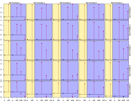
To give an idea about how regression coefficients of the FF3F model stack up against those of the CAPM for the 25 size/value sorted portfolios, I plotted the estimated parameters along with their significance in a similar plot as the returns plot above :

;

# TS Coefficients,Collective Plot
windows()
layout(matrix(c(1:25),nrow=5,ncol=5))
col1 &lt;- adjustcolor(col='gold',alpha.f=0.3)
col2 &lt;- adjustcolor(col='blue',alpha.f=0.3)
res.tot &lt;- NULL

for(i in 1:5){
  for(j in 1:5){
		coeff.matrix &lt;- cbind(BM.SZ$value.excess[[i]]$ts.alphas[j],BM.SZ$value.excess[[i]]$ts.betas[j],BM.SZ$value.excess[[i]]$ff.alphas[j],t(BM.SZ$value.excess[[i]]$ff.betas[,j]))
		res.tot &lt;- rbind(res.tot,coeff.matrix)
		pvalues.matrix &lt;- cbind(BM.SZ$value.excess[[i]]$capm.p.a[j],BM.SZ$value.excess[[i]]$capm.p.b[j],BM.SZ$value.excess[[i]]$ff.p.a[j],BM.SZ$value.excess[[i]]$ff.p.mkt[j],BM.SZ$value.excess[[i]]$ff.p.smb[j],BM.SZ$value.excess[[i]]$ff.p.hml[j])
		col.matrix&lt;-ifelse(pvalues.matrix&lt;0.05,'red','black')

		if(j==1 &amp;&amp; i&gt;1 &amp;&amp; i&lt;5)
		{
			par(mai=c(0.015,0.025,0.25,0.025))
		  plot(yaxt='n',xaxt='n',cex.main=0.85,cex.lab=0.65,cex.axis=0.65,x=1:length(coeff.matrix),coeff.matrix,type='h',col=col.matrix,lwd=1.5)
			points(x=1:length(coeff.matrix),y=coeff.matrix,col=col.matrix,cex=1,pch=19)
			abline(h=0)
			abline(v=2.5,col='darkred',lwd=1.5,lty=3)
			mtext(text=paste('BM Portfolios',i),side=3,cex=0.65)
			rect(0,-6,2.5,2,col=col1)
      rect(2.5,-6,7,2,col=col2)

		}
		else if(j&gt;1 &amp;&amp; j&lt;5 &amp;&amp; i&gt;1 &amp;&amp; i&lt;5)
		{
			par(mai=c(0.015,0.025,0.015,0.025))
		  plot(yaxt='n',xaxt='n',cex.main=0.85,cex.lab=0.65,cex.axis=0.65,x=1:length(coeff.matrix),coeff.matrix,type='h',col=col.matrix,lwd=1.5)
		  points(x=1:length(coeff.matrix),y=coeff.matrix,col=col.matrix,cex=1,pch=19)
			abline(h=0)
			abline(v=2.5,col='darkred',lwd=1.5,lty=3)
			rect(0,-6,2.5,2,col=col1)
      rect(2.5,-6,7,2,col=col2)

		}
		else if(j==1 &amp;&amp; i==1)
		{
			par(mai=c(0.015,0.25,0.25,0.025))
		  plot(xaxt='n',cex.main=0.85,cex.lab=0.65,cex.axis=0.65,x=1:length(coeff.matrix),coeff.matrix,type='h',col=col.matrix,lwd=1.5)
	    points(x=1:length(coeff.matrix),y=coeff.matrix,col=col.matrix,cex=1,pch=19)
			mtext(text=paste('BM Portfolios',i),side=3,cex=0.65)
			abline(h=0)
			abline(v=2.5,col='darkred',lwd=1.5,lty=3)
			rect(0,-6,2.5,2,col=col1)
      rect(2.5,-6,7,2,col=col2)

		}
		else if(j==1 &amp;&amp; i==5)
		{
			par(mai=c(0.015,0.025,0.25,0.15))
		  plot(yaxt='n',xaxt='n',cex.main=0.85,cex.lab=0.65,cex.axis=0.65,x=1:length(coeff.matrix),coeff.matrix,type='h',col=col.matrix,lwd=1.5)
			points(x=1:length(coeff.matrix),y=coeff.matrix,col=col.matrix,cex=1,pch=19)
			mtext(text=paste('Size Portfolios',j),side=4,cex=0.65)
			mtext(text=paste('BM Portfolios',i),side=3,cex=0.65)
			abline(h=0)
			abline(v=2.5,col='darkred',lwd=1.5,lty=3)
			rect(0,-6,2.5,2,col=col1)
      rect(2.5,-6,7,2,col=col2)

	}
		else if(j&gt;1 &amp;&amp; j&lt;5 &amp;&amp; i==1)
		{
		  par(mai=c(0.015,0.25,0.015,0.025))
		  plot(xaxt='n',cex.main=0.85,cex.lab=0.65,cex.axis=0.65,x=1:length(coeff.matrix),coeff.matrix,type='h',col=col.matrix,lwd=1.5)
      points(x=1:length(coeff.matrix),y=coeff.matrix,col=col.matrix,cex=1,pch=19)
			abline(h=0)
			abline(v=2.5,col='darkred',lwd=1.5,lty=3)
			rect(0,-6,2.5,2,col=col1)
      rect(2.5,-6,7,2,col=col2)

		}
		else if(j==5 &amp;&amp; i==1)
		{
			par(mai=c(0.25,0.25,0.015,0.025))
		  plot(xaxt='n',xlab='',cex.main=0.85,cex.lab=0.65,cex.axis=0.65,x=1:length(coeff.matrix),coeff.matrix,type='h',col=col.matrix,lwd=1.5)
    	axis(at=1:6,side=1,labels=c('a','mkt','a','mkt','smb','hml'))

			points(x=1:length(coeff.matrix),y=coeff.matrix,col=col.matrix,cex=1,pch=19)
			abline(h=0)
			abline(v=2.5,col='darkred',lwd=1.5,lty=3)
			rect(0,-6,2.5,2,col=col1)
      rect(2.5,-6,7,2,col=col2)

		}
		else if(j==5 &amp;&amp; i&gt;1 &amp;&amp; i&lt;5)
		{
			par(mai=c(0.25,0.025,0.015,0.025))
		  plot(xaxt='n',xlab='',yaxt='n',cex.main=0.85,cex.lab=0.65,cex.axis=0.65,x=1:length(coeff.matrix),coeff.matrix,type='h',col=col.matrix,lwd=1.5)
   		axis(at=1:6,side=1,labels=c('a','mkt','a','mkt','smb','hml'))

			points(x=1:length(coeff.matrix),y=coeff.matrix,col=col.matrix,cex=1,pch=19)
			abline(h=0)
			abline(v=2.5,col='darkred',lwd=1.5,lty=3)
			rect(0,-6,2.5,2,col=col1)
      rect(2.5,-6,7,2,col=col2)

		}
		else if(j==5 &amp;&amp; i==5)
		{
		 par(mai=c(0.25,0.025,0.015,0.15))
	   plot(xaxt='n',yaxt='n',cex.main=0.85,cex.lab=0.65,cex.axis=0.65,x=1:length(coeff.matrix),coeff.matrix,type='h',col=col.matrix,lwd=1.5)
     axis(at=1:6,side=1,labels=c('a','mkt','a','mkt','smb','hml'))

     points(x=1:length(coeff.matrix),y=coeff.matrix,col=col.matrix,cex=1,pch=19)
		 mtext(text=paste('Size Portfolio',j),cex=0.65,side=4)
		 abline(h=0)
		 abline(v=2.5,col='darkred',lwd=1.5,lty=3)
			rect(0,-6,2.5,2,col=col1)
      rect(2.5,-6,7,2,col=col2)

		}
		else if(j&gt;1 &amp;&amp; j&lt;5  &amp;&amp; i==5)
		{
		 par(mai=c(0.025,0.025,0.015,0.15))
	   plot(xaxt='n',yaxt='n',cex.main=0.85,cex.lab=0.65,cex.axis=0.65,x=1:length(coeff.matrix),coeff.matrix,type='h',col=col.matrix,lwd=1.5)

		 points(x=1:length(coeff.matrix),y=coeff.matrix,col=col.matrix,cex=1,pch=19)
     mtext(text=paste('Size Portfolio',j),cex=0.65,side=4)
		 abline(h=0)
		 abline(v=2.5,col='darkred',lwd=1.5,lty=3)
		 rect(0,-6,2.5,2,col=col1)
     rect(2.5,-6,7,2,col=col2)

		}
	}
}

aq

The yellow boxes cover CAPM estimates while the blue boxes cover FF parameters.Red lines indicate statistical significance at the 10% level, while black lines indicate non significance. For most portfolios the 3 risk factors tend to be significant and have the expected sign. As such, the smaller sized portfolios are more exposed to the SMB factor than larger sized portfolios. Exposure to the HML factor tends to increase as we move from growth to value stocks (left to right or B/M1 to B/M5). Clearly, the statistical significance of most of the factors points to the multifactor model being able to capture risk exposures beyond the conventional CAPM. It should be noted that the main point of the time series regression is NOT to explain stock returns but to see if the intercept term is low and if high average returns are associated with high slope parameters. Essentially, time series regressions provide the data for explaining stock returns, a task delegated to cross section regressions.

Starting with Keim(1981) and Banz(1981) in the early 1980s, a number of researchers found evidence that variation in firm size (defined as total market capitalisation) could help explain differences in expected returns, lending some empirical heft to the intuition that small stocks have a tendency to outperform large stocks.  In and of itself, the outperformance of small cap stocks does not violate the CAPM as long as average returns and systematic risk line up in a linear and positive manner as per theory. As such, statistically significant evidence of small stock portfolios systematically deviating positively from the fitted CAPM line, constituted a violation of the simple theory. This small firm effect,the tendency of small stock portfolios to earn a greater average return than larger stock portfolios, has been traditionally attributed to growth opportunities,fund corrections and volatile business environments that characterise many smaller firms as well as behavioural/psychological factors that beset investors.

Starting with Graham and Dodd in the late 1930s, a different line of inquiry was cast to investigate what is now termed the value effect. Value stocks tend to have market values that are small relative to their accounting book values and earn higher average returns than growth stocks which have less favourable book to market ratios. While value stocks are believed to be undervalued by the market and hence fetch significant positive expected returns when price corrections occur,growth stocks,also known as glamour stocks, tend to be overvalued by market participants and hence garner lower return expectations. Since violations of the CAPM typically constitute joint puzzles of expected returns and beta, it is useful to point out that the existence of high B/M (value) stocks with low prices and high expected returns is not a violation of the CAPM as long as these higher expected returns are justified by greater systematic risk. When perusing through some of the evidence found across various standard papers, there seems to be a hierarchy of violations, with an unexplained alpha (deviation of actual data from estimated relation) being the lesser of two evils when a negative relation between beta and average returns also emerges from the data. Hence finding an unexplained alpha is a less severe indictment of the CAPM than a negative risk-return relation. In the context of the value effect, there is nothing principally wrong about value stocks (high B/M) having higher returns than more expensive stocks (or stock groupings) as long as they also have higher betas to justify their higher expected returns. It is this absence of a positive risk return relationship that constitutes the value puzzle and hence a violation of the CAPM.

It should also be noted that the strength of both small firm and value effects are time dependent. The size effect appears to have vanished over the past 10-15 years.The value effect lined up surprisingly well with risk in the periods before 1963, the higher-beta-higher expected return relation fell through the cracks in periods after 1963 with growth stock portfolios being exposed to a level of systematic risk comparable to that of value portfolios without the disproportionate positive payoff that the latter enjoys. While the spread of returns between value and growth stocks may have been sensible on both sides of 1963, the betas did not line up with expected returns as required.

Motivated by the idea that value stocks and small firms may be exposed to sources of systematic risk not covered by the traditional CAPM beta, Fama and French (1993) specified a 3 factor model to account for this omission.

Before showing how the Fama/French 3 factor model  produces better explanations of expected returns than the single factor model (CAPM) , it is helpful to visualise some of the empirical facts that motivated the model in the first place. In the following section, monthly returns for the 25 size and value sorted portfolios are downloaded from the Kenneth French website,filtered for missing values and subsequently plotted in excess form against time. The subset of the data considered ranges from July 1963 to December 1993, the same period covered by the original authors.

Importing data from CSV file,dealing with missing values and subsetting data

#####################################################################################

#Import CSV file(s)
sz.bm.df <- read.csv('size_book_25.csv',header=T)
ff.df <- read.csv('Factor_data.csv',header=T)

#Deal with missing values
szbm.tot.data <- ts(data=sz.bm.df,start=c(1926,7),end=c(2012,12),frequency=12)
na.idx <- apply(szbm.tot.data == -99.99, 1, any)
sub.start <- time(szbm.tot.data)[tail(which(na.idx), 1)+1]
sub.end <- last(time(szbm.tot.data))
ff.tot.data <- ts(data=ff.df,start=c(1926,7),end=c(2012,12),frequency=12)/100

sub.c.1 <- c(1963,7)
sub.c.2 <- c(1993,12)

szbm.ts.data <- window(szbm.tot.data, start=sub.c.1,end=sub.c.2)/100

#Align FF factors,rf data to non-missing observations

exc.mkt <- window(ff.tot.data[,1],start=sub.c.1,end=sub.c.2)
smb.fct <- window(ff.tot.data[,2],start=sub.c.1,end=sub.c.2)
hml.fct <- window(ff.tot.data[,3],start=sub.c.1,end=sub.c.2)
rf.ret <- window(ff.tot.data[,4],start=sub.c.1,end=sub.c.2)

gh
Extracting portfolios from the subsetted data into list objects,time series regressions

for(i in 1:5){
  #Size focus
	SZ.BM$size.port[[i]] <- szbm.ts.data[,beg[i]:end[i]]
	SZ.BM$size.port.mean[[i]] <-matrix(colMeans(SZ.BM$size.port[[i]]),nrow=5)
	colnames(SZ.BM$size.port[[i]]) <- paste('Value',1:5)
	rownames(SZ.BM$size.port.mean[[i]]) <- paste ('Value',1:5)
	colnames(SZ.BM$size.port.mean[[i]]) <- paste ('Size',i)
	Returns.s <- rbind(Returns.s,SZ.BM$size.port.mean[[i]])

	#Value focus
	BM.SZ$value.port[[i]] <- szbm.ts.data[,beg+(i-1)]
  BM.SZ$value.port.mean[[i]] <-matrix(colMeans(BM.SZ$value.port[[i]]),nrow=5)
  colnames(BM.SZ$value.port[[i]]) <- paste('Size',1:5)
	rownames(BM.SZ$value.port.mean[[i]]) <- paste ('Size',1:5)
	colnames(BM.SZ$value.port.mean[[i]]) <- paste ('Value',i)
	Returns.v <- rbind(Returns.v,BM.SZ$value.port.mean[[i]])

	#Excess Size focus,regressions
	SZ.BM$size.excess[[i]] <- SZ.BM$size.port[[i]]-rf.ret
		colnames(SZ.BM$size.excess[[i]]) <- paste('Value',1:5)

	##time series capm
	  s.temp <- SZ.BM$size.excess[[i]]
		SZ.BM$size.excess[[i]]$ts.obj <- lm(s.temp~exc.mkt)
		SZ.BM$size.excess[[i]]$ts.alphas <- as.matrix(coef(SZ.BM$size.excess[[i]]$ts.obj)[1,])
		SZ.BM$size.excess[[i]]$ts.betas <- as.matrix(coef(SZ.BM$size.excess[[i]]$ts.obj)[2,])
	  SZ.BM$size.excess[[i]]$ts.fitted <- fitted(SZ.BM$size.excess[[i]]$ts.obj)
	  s.betas[[i]] <- SZ.BM$size.excess[[i]]$ts.betas

	##time series FF
    SZ.BM$size.excess[[i]]$ff.obj <- lm(s.temp~exc.mkt+smb.fct+hml.fct)
		SZ.BM$size.excess[[i]]$ff.alphas <- as.matrix(coef(SZ.BM$size.excess[[i]]$ff.obj)[1,])
		SZ.BM$size.excess[[i]]$ff.betas <- as.matrix(coef(SZ.BM$size.excess[[i]]$ff.obj)[2:4,])
	  SZ.BM$size.excess[[i]]$ff.fitted <- fitted(SZ.BM$size.excess[[i]]$ff.obj)
	  s.ff.betas[[i]] <- SZ.BM$size.excess[[i]]$ff.betas

	#Excess Value focus,regressions
	BM.SZ$value.excess[[i]] <- BM.SZ$value.port[[i]]-rf.ret
		colnames(BM.SZ$value.excess[[i]]) <- paste('Size',1:5)

	##time series capm
	  v.temp <- BM.SZ$value.excess[[i]]
		BM.SZ$value.excess[[i]]$ts.obj <- lm(v.temp~exc.mkt)
		BM.SZ$value.excess[[i]]$ts.alphas <- as.matrix(coef(BM.SZ$value.excess[[i]]$ts.obj)[1,])
		BM.SZ$value.excess[[i]]$ts.betas <- as.matrix(coef(BM.SZ$value.excess[[i]]$ts.obj)[2,])
	  BM.SZ$value.excess[[i]]$ts.fitted <- fitted(BM.SZ$value.excess[[i]]$ts.obj)
	  v.betas[[i]] <- BM.SZ$value.excess[[i]]$ts.betas

		##time series FF
    BM.SZ$value.excess[[i]]$ff.obj <- lm(v.temp~exc.mkt+smb.fct+hml.fct)
		BM.SZ$value.excess[[i]]$ff.alphas <- as.matrix(coef(BM.SZ$value.excess[[i]]$ff.obj)[1,])
		BM.SZ$value.excess[[i]]$ff.betas <- as.matrix(coef(BM.SZ$value.excess[[i]]$ff.obj)[2:4,])
	  BM.SZ$value.excess[[i]]$ff.fitted <- fitted(BM.SZ$value.excess[[i]]$ff.obj)
	  v.ff.betas[[i]] <- BM.SZ$value.excess[[i]]$ff.betas

	##cross section capm
    cb <- colMeans(v.temp)
  	BM.SZ$value.excess.avg[[i]] <- cb
	  coeff3.rhs <- matrix(v.betas[[i]])
    BM.SZ$value.excess.avg[[i]]$cs.obj <- lm(cb~coeff3.rhs)
		BM.SZ$value.excess[[i]]$cs.alphas <- as.matrix(coef(BM.SZ$value.excess.avg[[i]]$cs.obj)[1])
		BM.SZ$value.excess[[i]]$cs.betas <- as.matrix(coef(BM.SZ$value.excess.avg[[i]]$cs.obj)[2])
	  BM.SZ$value.excess[[i]]$cs.fitted <- fitted(BM.SZ$value.excess.avg[[i]]$cs.obj)

  ##cross section ff
	  cs2.temp <- colMeans(v.temp)
	  BM.SZ$value.avg.ff[[i]] <- cs2.temp
	  coeff4.rhs <- matrix(t(v.ff.betas[[i]]),ncol=3)
    BM.SZ$value.avg.ff[[i]]$cs.obj <- lm(cs2.temp~coeff4.rhs)
		BM.SZ$value.avg.ff[[i]]$cs.alphas <- as.matrix(coef(BM.SZ$value.avg.ff[[i]]$cs.obj)[1])
		BM.SZ$value.avg.ff[[i]]$cs.betas <- as.matrix(coef(BM.SZ$value.avg.ff[[i]]$cs.obj)[2:4])
	  BM.SZ$value.avg.ff[[i]]$cs.fitted <- fitted(BM.SZ$value.avg.ff[[i]]$cs.obj)

	##Rsquared;pvalue
		SZ.BM$size.excess[[i]]$capm.p.a <- NULL
		SZ.BM$size.excess[[i]]$capm.p.b <- NULL

		BM.SZ$value.excess[[i]]$capm.p.a <- NULL
		BM.SZ$value.excess[[i]]$capm.p.b <- NULL

		SZ.BM$size.excess[[i]]$capm.rsq <- NULL
		BM.SZ$value.excess[[i]]$capm.rsq <- NULL

		SZ.BM$size.excess[[i]]$ff.p.a <- NULL
		SZ.BM$size.excess[[i]]$ff.p.mkt <- NULL
		SZ.BM$size.excess[[i]]$ff.p.smb <- NULL
		SZ.BM$size.excess[[i]]$ff.p.hml <- NULL

		SZ.BM$size.excess[[i]]$ff.rsq <- NULL

	  BM.SZ$value.excess[[i]]$ff.p.a <- NULL
		BM.SZ$value.excess[[i]]$ff.p.mkt <- NULL
		BM.SZ$value.excess[[i]]$ff.p.smb <- NULL
		BM.SZ$value.excess[[i]]$ff.p.hml <- NULL

		BM.SZ$value.excess[[i]]$ff.rsq <- NULL

	  for(j in 1:5){
	  	#capm.p
	  	SZ.BM$size.excess[[i]]$capm.p.a <- cbind(SZ.BM$size.excess[[i]]$capm.p.a,summary(SZ.BM$size.excess[[i]]$ts.obj)[[j]][[4]][1,4])
	  	SZ.BM$size.excess[[i]]$capm.p.b <- cbind(SZ.BM$size.excess[[i]]$capm.p.b,summary(SZ.BM$size.excess[[i]]$ts.obj)[[j]][[4]][2,4])
	  	BM.SZ$value.excess[[i]]$capm.p.a <- cbind(SZ.BM$size.excess[[i]]$capm.p.a,summary(BM.SZ$value.excess[[i]]$ts.obj)[[j]][[4]][1,4])
	  	BM.SZ$value.excess[[i]]$capm.p.b <- cbind(SZ.BM$size.excess[[i]]$capm.p.b,summary(BM.SZ$value.excess[[i]]$ts.obj)[[j]][[4]][2,4])

	  	#ff.p
	  	SZ.BM$size.excess[[i]]$ff.p.a <- cbind(SZ.BM$size.excess[[i]]$ff.p.a,summary(SZ.BM$size.excess[[i]]$ff.obj)[[j]][[4]][1,4])
	  	SZ.BM$size.excess[[i]]$ff.p.mkt <- cbind(SZ.BM$size.excess[[i]]$ff.p.mkt,summary(SZ.BM$size.excess[[i]]$ff.obj)[[j]][[4]][2,4])
	  	SZ.BM$size.excess[[i]]$ff.p.smb <- cbind(SZ.BM$size.excess[[i]]$ff.p.smb,summary(SZ.BM$size.excess[[i]]$ff.obj)[[j]][[4]][3,4])
	  	SZ.BM$size.excess[[i]]$ff.p.hml <- cbind(SZ.BM$size.excess[[i]]$ff.p.hml,summary(SZ.BM$size.excess[[i]]$ff.obj)[[j]][[4]][2,4])

	  	BM.SZ$value.excess[[i]]$ff.p.a <- cbind(BM.SZ$value.excess[[i]]$ff.p.a,summary(BM.SZ$value.excess[[i]]$ff.obj)[[j]][[4]][1,4])
	  	BM.SZ$value.excess[[i]]$ff.p.mkt <- cbind(BM.SZ$value.excess[[i]]$ff.p.mkt,summary(BM.SZ$value.excess[[i]]$ff.obj)[[j]][[4]][2,4])
	  	BM.SZ$value.excess[[i]]$ff.p.smb <- cbind(BM.SZ$value.excess[[i]]$ff.p.smb,summary(BM.SZ$value.excess[[i]]$ff.obj)[[j]][[4]][3,4])
	  	BM.SZ$value.excess[[i]]$ff.p.hml <- cbind(BM.SZ$value.excess[[i]]$ff.p.hml,summary(BM.SZ$value.excess[[i]]$ff.obj)[[j]][[4]][4,4])

	  	#Rsq
	  	SZ.BM$size.excess[[i]]$capm.rsq <- cbind(SZ.BM$size.excess[[i]]$capm.rsq,summary(SZ.BM$size.excess[[i]]$ts.obj)[[j]][[9]])
	  	BM.SZ$value.excess[[i]]$capm.rsq <- cbind(BM.SZ$value.excess[[i]]$capm.rsq,summary(BM.SZ$value.excess[[i]]$ts.obj)[[j]][[9]])

	  	SZ.BM$size.excess[[i]]$ff.rsq <- cbind(SZ.BM$size.excess[[i]]$ff.rsq,summary(SZ.BM$size.excess[[i]]$ff.obj)[[j]][[9]])
	  	BM.SZ$value.excess[[i]]$ff.rsq <- cbind(BM.SZ$value.excess[[i]]$ff.rsq,summary(BM.SZ$value.excess[[i]]$ff.obj)[[j]][[9]])

	  }
}

k
Clearly it would have been better to embed these in separate functions,but I cannot be bothered right now. Also for some inexplicable reason, the copied code does not align as it used to in previous posts on this blog.

To visualise the collective time series plots of the 25 portfolios :

#Collective Plots for excess returns
port.exc <- list()
col.bar <- adjustcolor(col='gold',alpha.f=0.65)
col.bar2 <- adjustcolor(col='white',alpha.f=0.5)

windows()
layout(matrix(c(1:25),nrow=5,ncol=5))
for(i in 1:5){
  port.exc[[i]] <- BM.SZ$value.port[[i]]-rf.ret
	for(j in 1:5){
		if(j==1 && i>1 && i<5)
		{
			par(mai=c(0.015,0.025,0.25,0.025))
		  plot(yaxt='n',xaxt='n',cex.main=0.85,cex.lab=0.65,cex.axis=0.65,port.exc[[i]][,j])
			mtext(text=paste('BM Portfolios',i),side=3,cex=0.65)
			abline(h=mean(port.exc[[i]][,j]),col=col.bar,lwd=round(mean(port.exc[[i]][,j])*600))
			abline(h=mean(port.exc[[i]][,j]),col=col.bar2,lwd=round(mean(port.exc[[i]][,j])*250))

			legend('topright',fill=col.bar,legend=paste('Mean',round(mean(port.exc[[i]][,j]),5)*100),ncol=1,bg='white',bty='n',cex=0.6)
		}
		else if(j>1 && j<5 && i>1 && i<5)
		{
			par(mai=c(0.015,0.025,0.015,0.025))
		  plot(yaxt='n',xaxt='n',cex.main=0.85,cex.lab=0.65,cex.axis=0.65,port.exc[[i]][,j])
			abline(h=mean(port.exc[[i]][,j]),col=col.bar,lwd=round(mean(port.exc[[i]][,j])*600))
			abline(h=mean(port.exc[[i]][,j]),col=col.bar2,lwd=round(mean(port.exc[[i]][,j])*250))

			legend('topright',fill=col.bar,legend=paste('Mean',round(mean(port.exc[[i]][,j]),5)*100),ncol=1,bg='white',bty='n',cex=0.6)
		}
		else if(j==1 && i==1)
		{
			par(mai=c(0.015,0.25,0.25,0.025))
		  plot(xaxt='n',cex.main=0.85,cex.lab=0.65,cex.axis=0.65,port.exc[[i]][,j])
			mtext(text=paste('BM Portfolios',i),side=3,cex=0.65)
			abline(h=mean(port.exc[[i]][,j]),col=col.bar)
			abline(h=mean(port.exc[[i]][,j]),col=col.bar2,lwd=round(mean(port.exc[[i]][,j])*250))

			legend('topright',fill=col.bar,legend=paste('Mean',round(mean(port.exc[[i]][,j]),5)*100),ncol=1,bg='white',bty='n',cex=0.6)
		}
		else if(j==1 && i==5)
		{
			par(mai=c(0.015,0.025,0.25,0.15))
		  plot(yaxt='n',xaxt='n',cex.main=0.85,cex.lab=0.65,cex.axis=0.65,port.exc[[i]][,j])
			mtext(text=paste('Size Portfolios',j),side=4,cex=0.65)
			mtext(text=paste('BM Portfolios',i),side=3,cex=0.65)
			abline(h=mean(port.exc[[i]][,j]),col=col.bar,lwd=round(mean(port.exc[[i]][,j])*600))
			abline(h=mean(port.exc[[i]][,j]),col=col.bar2,lwd=round(mean(port.exc[[i]][,j])*250))

			legend('topright',fill=col.bar,legend=paste('Mean',round(mean(port.exc[[i]][,j]),5)*100),ncol=1,bg='white',bty='n',cex=0.6)
		}
		else if(j>1 && j<5 && i==1)
		{
		  par(mai=c(0.015,0.25,0.015,0.025))
		  plot(xaxt='n',cex.main=0.85,cex.lab=0.65,cex.axis=0.65,port.exc[[i]][,j])
			abline(h=mean(port.exc[[i]][,j]),col=col.bar,lwd=round(mean(port.exc[[i]][,j])*600))
			abline(h=mean(port.exc[[i]][,j]),col=col.bar2,lwd=round(mean(port.exc[[i]][,j])*250))

			legend('topright',fill=col.bar,legend=paste('Mean',round(mean(port.exc[[i]][,j]),5)*100),ncol=1,bg='white',bty='n',cex=0.6)
		}
		else if(j==5 && i==1)
		{
			par(mai=c(0.25,0.25,0.015,0.025))
		  plot(xlab='',cex.main=0.85,cex.lab=0.65,cex.axis=0.65,port.exc[[i]][,j])
			abline(h=mean(port.exc[[i]][,j]),col=col.bar,lwd=round(mean(port.exc[[i]][,j])*600))
			abline(h=mean(port.exc[[i]][,j]),col=col.bar2,lwd=round(mean(port.exc[[i]][,j])*250))

			legend('topright',fill=col.bar,legend=paste('Mean',round(mean(port.exc[[i]][,j]),5)*100),ncol=1,bg='white',bty='n',cex=0.6)
		}
		else if(j==5 && i>1 && i<5)
		{
			par(mai=c(0.25,0.025,0.015,0.025))
		  plot(xlab='',yaxt='n',cex.main=0.85,cex.lab=0.65,cex.axis=0.65,port.exc[[i]][,j])
			abline(h=mean(port.exc[[i]][,j]),col=col.bar,lwd=round(mean(port.exc[[i]][,j])*600))
			abline(h=mean(port.exc[[i]][,j]),col=col.bar2,lwd=round(mean(port.exc[[i]][,j])*250))

			legend('topright',fill=col.bar,legend=paste('Mean',round(mean(port.exc[[i]][,j]),5)*100),ncol=1,bg='white',bty='n',cex=0.6)
		}
		else if(j==5 && i==5)
		{
		 par(mai=c(0.25,0.025,0.015,0.15))
	   plot(yaxt='n',cex.main=0.85,cex.lab=0.65,cex.axis=0.65,port.exc[[i]][,j])
     mtext(text=paste('Size Portfolio',j),cex=0.65,side=4)
		 abline(h=mean(port.exc[[i]][,j]),col=col.bar,lwd=round(mean(port.exc[[i]][,j])*600))
		 abline(h=mean(port.exc[[i]][,j]),col=col.bar2,lwd=round(mean(port.exc[[i]][,j])*250))

		 legend('topright',fill=col.bar,legend=paste('Mean',round(mean(port.exc[[i]][,j]),5)*100),ncol=1,bg='white',bty='n',cex=0.6)
		}
		else if(j>1 && j<5  && i==5)
		{
		 par(mai=c(0.025,0.025,0.015,0.15))
	   plot(xaxt='n',yaxt='n',cex.main=0.85,cex.lab=0.65,cex.axis=0.65,port.exc[[i]][,j])
     mtext(text=paste('Size Portfolio',j),cex=0.65,side=4)
		 abline(h=mean(port.exc[[i]][,j]),col=col.bar,lwd=round(mean(port.exc[[i]][,j])*600))
		 abline(h=mean(port.exc[[i]][,j]),col=col.bar2,lwd=round(mean(port.exc[[i]][,j])*250))

			legend('topright',fill=col.bar,legend=paste('Mean',round(mean(port.exc[[i]][,j]),5)*100),ncol=1,bg='white',bty='n',cex=0.6)
		}
	}
}

g

This generates the following plot along with a high quality image here

gg


This collective plot charts excess monthly returns across the 25 portfolios. The yellow line is simply the mean return associated with each portfolio scaled to visualise return differences. Size portfolio 1 is a collection of the smallest stocks while BM portfolio 1 is a collection of stocks with the lowest book-to-market ratios (growth stocks). Hence horizontal movements starting from the left mimics moving along the growth/value spectrum and vertical movements starting from the top mimics moving along the small cap/large cap spectrum.  Holding size constant, mean returns tend to increase as we move toward value stocks and away from growth stocks. Holding value constant,mean returns tend to decrease as we move toward large stocks and away from small stocks. Hence the greatest mean return comes from holding small size value stocks (top right corner),visually corroborated by the plot having the widest yellow bar.  

Fama and MacBeth (1973) suggest an alternative procedure for running cross-sectional regressions. The first step of the procedure is identical to the time series regression performed earlier, where excess asset returns were regressed against excess market returns. The estimates of  beta are then fed as inputs into a cross section regression which constitutes the second step of the FMB process. The difference between the two pass regression examined in the previous blog posts and the FMB procedure delineated here is that the latter estimates a cross-sectional regression at each time period while the former estimates a single cross-sectional regression with sample averages.

This post focuses on the application of the FMB methodology to the previous dataset.

[1] Estimate a beta for each of the 351 stocks on the basis of the first 48 months of observations in the data set.

[2] Rank order all of the stock betas, and form 20 portfolios with assets appearing in descending order in terms of their systematic risk.

[3]Estimate a portfolio beta for each of the 20 portfolios by regressing portfolio monthly returns against excess market returns on the basis of the next 60 months worth of observations.

[4] Estimate the expost SML for each month of the next 48 months worth of data.

[5] Estimate the SML accounting for nonlinearity and residual variances for the same time period as step 4.

[6] Repeat steps 1-5 as often as possible across adjacent regression windows. Unfortunately in this case,due to data restrictions, I only have 2 regression windows before running out of data.

[7] Compute the mean value for each of the coefficients estimated in steps 5 and 6.

The code for the FMB procedure follows

#Fama MacBeth
FB <- list()
 
  alpha.list <- NULL
  beta.list <- NULL
 
  nl.alpha.list <- NULL
  nl.beta.list <- NULL
  nl.betasq.list <- NULL
 
  rv.alpha.list <- NULL
  rv.beta.list <- NULL
  rv.betasq.list <- NULL
  rv.res.list <- NULL
 
  FB$windows1.loc.beg <- c(1,49)
  FB$windows1.loc.end <- c(48,96)
 
  FB$windows2.loc.beg <- c(49,97)
  FB$windows2.loc.end <- c(108,156)
 
  FB$windows3.loc.beg <- c(109,157)
  FB$windows3.loc.end <- c(156,204)
 
  FB$port.beg <- c(seq(1,289,by=18),seq(307,337,by=15))
  FB$port.end <- c(seq(18,306,by=18),seq(321,351,by=15))
 
  FB$num.windows <- 2
	
  FB$windows <- list()
 
        for(i in 1:FB$num.windows){
         FB$windows[[i]]<-list()
         FB$windows[[i]]$alpha.list <- NULL
	 FB$windows[[i]]$beta.list <- NULL
	 FB$windows[[i]]$portfolios <- NULL
	 FB$windows[[i]]$portfolios.mean <- NULL			
         FB$windows[[i]]$portfolio.mat <- NULL
         FB$windows[[i]]$port.fit <- NULL
			
	for(j in 1:ncol(stock.ret)){
	 FB$windows[[i]]$fit[[j]]<-lm(ex.ret[FB$windows1.loc.beg[i]:FB$windows1.loc.end[i],j]~exm.ret[FB$windows1.loc.beg[i]:FB$windows1.loc.end[i]]) 
	 FB$windows[[i]]$fit[[j]]$alpha <- coef(FB$windows[[i]]$fit[[j]])[1]
         FB$windows[[i]]$fit[[j]]$beta <- coef(FB$windows[[i]]$fit[[j]])[2]
			  
         FB$windows[[i]]$alpha.list <- rbind(FB$windows[[i]]$alpha.list,FB$windows[[i]]$fit[[j]]$alpha)
	 FB$windows[[i]]$beta.list <- rbind(FB$windows[[i]]$beta.list,FB$windows[[i]]$fit[[j]]$beta)
				
	 FB$windows[[i]]$fit[[j]]$alpha.p <- summary(FB$windows[[i]]$fit[[j]])[[4]][7]
	 FB$windows[[i]]$fit[[j]]$beta.p <- summary(FB$windows[[i]]$fit[[j]])[[4]][8]
			  
	 FB$windows[[i]]$fit[[j]]$rsquared <- summary(FB$windows[[i]]$fit[[j]])[[9]]
	}
			
	rownames(FB$windows[[i]]$alpha.list) <- colnames(monthly.ret)
	rownames(FB$windows[[i]]$beta.list) <- colnames(monthly.ret)
	colnames(FB$windows[[i]]$alpha.list) <- 'alphas'
	colnames(FB$windows[[i]]$beta.list) <- 'betas'
			
	FB$windows[[i]]$matrix <- cbind(FB$windows[[i]]$alpha.list,FB$windows[[i]]$beta.list,t(stock.ret[(FB$windows2.loc.beg[i]):(FB$windows2.loc.end[i]),1:351]))
	FB$windows[[i]]$matrix.sorted <- FB$windows[[i]]$matrix[order(FB$windows[[i]]$matrix[,2],decreasing=TRUE),]
			
	for(k in 1:20){
	 FB$windows[[i]]$portfolios[[k]] <- FB$windows[[i]]$matrix.sorted[FB$port.beg[k]:FB$port.end[k],]
	 FB$windows[[i]]$portfolios.mean[[k]] <- matrix(colMeans(FB$windows[[i]]$portfolios[[k]][,3:62]),ncol=1)
	 FB$windows[[i]]$portfolio.mat <- cbind(FB$windows[[i]]$portfolio.mat,FB$windows[[i]]$portfolios.mean[[k]])
	}
 
	colnames(FB$windows[[i]]$portfolio.mat) <- paste('Portfolio ',1:20)
      	FB$windows[[i]]$port.fit <- lm(FB$windows[[i]]$portfolio.mat~exm.ret[FB$windows2.loc.beg[i]:FB$windows2.loc.end[i],1])
        FB$windows[[i]]$port.betas <- matrix(coef(FB$windows[[1]]$port.fit)[2,],ncol=1)
	FB$windows[[i]]$matrix.sml <- cbind(FB$windows[[i]]$alpha.list,FB$windows[[i]]$beta.list,t(stock.ret[(FB$windows3.loc.beg[i]):(FB$windows3.loc.end[i]),1:351]))
	FB$windows[[i]]$matrix.sorted.sml <- FB$windows[[i]]$matrix.sml[order(FB$windows[[i]]$matrix.sml[,2],decreasing=TRUE),]
			
	for(k in 1:20){
	 FB$windows[[i]]$portfolios.sml[[k]] <- FB$windows[[i]]$matrix.sorted.sml[FB$port.beg[k]:FB$port.end[k],]
	 FB$windows[[i]]$portfolios.mean.sml[[k]] <- matrix(colMeans(FB$windows[[i]]$portfolios.sml[[k]][,3:50]),ncol=1)
	 FB$windows[[i]]$portfolio.mat.sml <- (cbind(FB$windows[[i]]$portfolio.mat.sml,FB$windows[[i]]$portfolios.mean.sml[[k]]))
	}	
	FB$windows[[i]]$portfolio.mat.sml<-t(FB$windows[[i]]$portfolio.mat.sml)
        FB$windows[[i]]$portfolio.sml.fit <- lm(FB$windows[[i]]$portfolio.mat.sml~FB$windows[[i]]$port.betas)
	sq <- ((FB$windows[[i]]$port.betas)^2)
	resd <- apply(resid(FB$windows[[i]]$port.fit),2,sd)^2
			
        FB$windows[[i]]$portfolio.nonl.fit <- lm(FB$windows[[i]]$portfolio.mat.sml~FB$windows[[i]]$port.betas+sq)
        FB$windows[[i]]$portfolio.rv.fit <- lm(FB$windows[[i]]$portfolio.mat.sml~FB$windows[[i]]$port.betas+sq+resd)
 
	alpha.list <- rbind(alpha.list,matrix(ncol=1,coef(FB$windows[[i]]$portfolio.sml.fit)[1,]))
        alpha.mean <- mean(alpha.list)
			
	beta.list <- rbind(beta.list,matrix(ncol=1,coef(FB$windows[[i]]$portfolio.sml.fit)[2,]))
        beta.mean <- mean(beta.list)
			
	nl.alpha.list <- rbind(nl.alpha.list,matrix(ncol=1,coef(FB$windows[[i]]$portfolio.nonl.fit)[1,]))
        nl.alpha.mean <- mean(nl.alpha.list)
		
	nl.beta.list <- rbind(nl.beta.list,matrix(ncol=1,coef(FB$windows[[i]]$portfolio.nonl.fit)[2,]))
        nl.beta.mean <- mean(nl.beta.list)
 
	nl.betasq.list <- rbind(nl.betasq.list,matrix(ncol=1,coef(FB$windows[[i]]$portfolio.nonl.fit)[3,]))
        nl.betasq.mean <- mean(nl.betasq.list)
			
	rv.alpha.list <- rbind(rv.alpha.list,matrix(ncol=1,coef(FB$windows[[i]]$portfolio.rv.fit)[1,]))
        rv.alpha.mean <- mean(rv.alpha.list)
		
	rv.beta.list <- rbind(rv.beta.list,matrix(ncol=1,coef(FB$windows[[i]]$portfolio.rv.fit)[2,]))
        rv.beta.mean <- mean(rv.beta.list)
 
	rv.betasq.list <- rbind(rv.betasq.list,matrix(ncol=1,coef(FB$windows[[i]]$portfolio.rv.fit)[3,]))
        rv.betasq.mean <- mean(rv.betasq.list)
 
        rv.res.list <- rbind(rv.res.list,matrix(ncol=1,coef(FB$windows[[i]]$portfolio.rv.fit)[4,]))
        rv.res.mean <- mean(rv.res.list)
}

Clearly the BJS and FMB procedures have been hardcoded for the current example rather than generalised for any arbitrary dataset.

To visualise some of the results

#Visualise FB
tab1 tab2 annot c1 c2 tab
port.names for(k in 1:17){
  port.names   port.names }

for(k in 18:20){
  port.names  port.names }

tab.port rn tab.port annot.port
windows()
layout(matrix(c(1,1,1,2,2),nrow=5,ncol=1))

par(mai=c(0,0,0.2,0))
TableMaker(row.h=c(1),apply(tab.port,2,rev),annot.port,strip=F,strip.col=c('red','green'),col.cut=0,alpha=0.6,border.col='lightgrey',text.col='black',header.bcol='gold',header.tcol='black',title='Portfolios in window 1')

par(mai=c(0.55,0.55,0.2,0.2))
colours plot(xlab='months',ylab='portfolio mean returns',main='Mean portfolio returns for next 5 years',cex.main=0.85,cex.lab=0.8,cex.axis=0.8,as.ts(FB$windows[[1]]$portfolios.mean[[1]]),col=colours[1])
for(i in 2:20){
	lines(FB$windows[[1]]$portfolios.mean[[i]],col=colours[i])
}
legend('top',fill=colours,legend=paste('Portfolio',1:20),ncol=10,bg='white',bty='n',cex=0.6)

annot r1 tab.com1 tab.com2 tab.com2
windows()
par(mai=c(0,0,0,0))
TableMaker(row.h=c(1),apply(tab.com1,2,rev),annot,strip=F,strip.col=c('red','green'),col.cut=0,alpha=0.6,border.col='white',text.col='black',header.bcol='light blue',header.tcol='black',title='Portfolios in window 1')

windows()
par(mai=c(0,0,0,0))
TableMaker(row.h=c(1),apply(tab.com2,2,rev),annot,strip=F,strip.col=c('red','green'),col.cut=0,alpha=0.6,border.col='white',text.col='black',header.bcol='light blue',header.tcol='black',title='Portfolios in window 1')

To get a sense of how the 20 beta-sorted portfolios look like, i have plotted their composition in the following table. Rows signify portfolios, with the smaller numbered portfolios corresponding to collections of assets with higher betas and larger numbered portfolios corresponding to collections of assets with lower betas. Since we have 351 assets in our dataset, we cannot evenly divide them into 20 equally sized portfolios. As a consequence, the first 17 portfolios have 18 assets while the last three portfolios have 15 assets in order to,quite arbitrarily, cover the total of 351 assets. The data plotted here is for the first regression window,covering the first 48 months of observations. The next and final regression window would cover the next 48 months of data (not shown here). The line chart at the bottom of the plot window tracks the average return of each of the 20 portfolios over the next 60 months in the dataset. This corresponds to step 3 of the FMB process outlined above.

nm

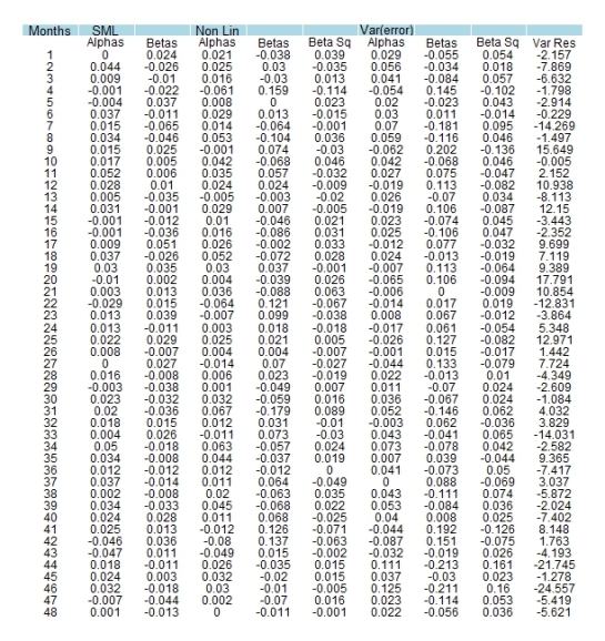
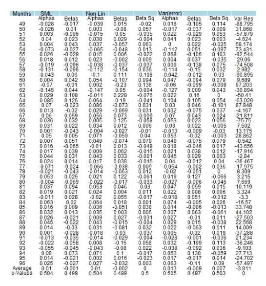
To get a sense of the coefficient estimates from steps 4-6, the following table (splitted into two plots due to plotting space problems) summarises estimated parameters for 3 models across two regression windows that total 96 months of data (48 months of observations per window).

mnh

The last rows of the table reflect column averages and associated p-values, which taken together should inform CAPM consistency. The only time we can reject the null hypothesis is with respect to residual variances in the last model such that for all other figures, statistical insignificance is to be inferred. Alphas, being statistically indistinguishable from 0 at traditional levels of significance is a point towards the CAPM.Betas,being insignificant do not help in explaining portfolio returns,constitute a departure from theory . Nonlinearity does not seem to be an issue but residual variance appears to matter greatly.On balance the CAPM does not seem to hold in terms of its implications for beta and residual variances but appears somewhat sensible for alphas and nonlinearity.