Asset Pricing [9a : Regime Switching]

In this series of posts I intend to replicate some of the methodologies applied by Kritzman et al.(2012) in their paper – Regime Shifts: Implications for Dynamic Strategies – , wherein :

• a two-state hidden Markov model is fitted to observed (or transformed) measures of financial turbulence,inflation and economic growth to partition history into meaningful regimes .
• the in-sample performance of a variety of risk premia is probed by comparing scaled differences in respective state means across regime variables.
• the out-of-sample performance of risk premia is examined by [1] tilting portfolios dynamically according to the likelihood of a particular regime and by [2] comparing the results of asset allocation that is conscious of regime switching versus the static alternative.

The excellent (but sadly idle) Quantivity blog has replicated some parts of the paper with much more rigour than I am capable of. This is perhaps as good a time as any to mention some differences between my post,the original paper and Quantivity’s post (QP).

One point of departure between my and QP’s post relates to the library/package used to estimate the hidden markov model. While QP used the RHmm package, I can only use the depmixS4 package (RHmm seems to be incompatible with newer versions of R…at least for me). As far as I can tell,the depmixS4 package does not support forecasting which means that I will probably not be able to take a gander at the out-of-sample issues alluded to above.

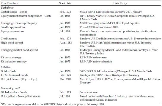
Another difference relates to the risk premia used in the original paper versus my post.

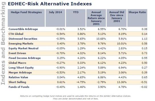
Instead of using these data series (shamelessly snipped from the paper), I simply downloaded a revised edhec data set (which comes with the PerformanceAnalytics package) from the edhec-risk-homepage : http://www.edhec-risk.com/indexes/pure_style. 

These are simply returns on various hedge fund strategies as opposed to deliberately constructed risk premia that are expected to respond to different states across economic/financial regime variables. A snapshot of the strategies follows, along with their most recent summary results :

 

---

 

[Data]

In terms of the data used in this project, it is useful to make a distinction at the outset between economic regime variables which are used to partition history into different states in a meaningful way) and risk premia (simple returns in my case) which are used to assess performance across states for each economic regime variable.

 

–Economic Regime Variables–

[1] Financial Market Turbulence

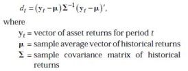
The paper defines this variable as a condition in which asset prices behave in an unusual fashion given historical patterns of behaviour and proposes to measure it using the Mahalanobis distance :

Financial market turbulence comes in two flavours : Equity and Foreign exchange.

The Equity Turbulence Index (ETI) was constructed by [1] downloading sp500 daily returns,[2] estimating mean and covariances using equally weighted historical returns for the past 10 years and [3] averaging the daily turbulence scores within each month. The Currency Turbulence Index (CTI) was constructed by [1] downloading daily currency returns (vs.USD) for 8 of the G-10 countries, [2] estimating mean and covariances using equally weighted historical returns for the past 3 years and [3] averaging the daily turbulence scores within each month.

The code for downloading relevant time series follows :

######################[a] Economic Regime Variables######################################

#[a.1] Equity Turbulence
symbol <- c('^GSPC')
beg <- as.Date('1970/01/01')
end <- as.Date('2014/01/01')

getSymbols(symbol,from=beg,to=end)
SPX.ret <- ROC(eval(parse(text=paste(substr(symbol,start=which(strsplit(symbol,split='^')[[1]]=='^')+1,stop=nchar(symbol)),'$GSPC.Close',sep=''))),n=1)
attr(SPX.ret,'type')='Equity'

#[a.2] Currency Turbulence
G9curr <- c('DEXUSAL','DEXUSUK','DEXCAUS','DEXNOUS','DEXJPUS','DEXUSNZ','DEXSDUS','DEXSZUS')
col.xts <- c('AUS','GBP','CAD','NOR','JAP','NZD','SWD','CHF')
inverted.idx <- grep('DEXUS',G9curr,value=F)
normal.idx <- index(G9curr)[-inverted.idx]

getSymbols(G9curr,src='FRED')
fx.xts <- do.call(merge,lapply(G9curr,function(x) eval(parse(text=x))))
names(fx.xts) <- col.xts

for(i in inverted.idx) fx.xts[,i] <- 1/eval(parse(text=G9curr[i]))
fx.xts <- ROC(fx.xts)
attr(fx.xts,'type')='Currency'

lI

[2] Inflation

Inflation was measured using the Consumer Price Index For All Urban Consumers :All Items, available from the FRED website and directly accessible via r :

#[a.3] Inflation Turbulence
getSymbols('CPIAUCNS',src='FRED')
inf.xts <- ROC(CPIAUCNS['1946-01-01::',1],n=1)
attr(inf.xts,'type')='Inflation'

l
[3] Economic Growth

Economic growth was measured using quarterly percentage growth in Real Gross Domestic Product :

#[a.4] Economic growth Turbulence
getSymbols('GDPC1',src='FRED')
ecg.xts <- ROC(GDPC1['1947-01-01::',1],n=1)
attr(ecg.xts,'type')='Growth'

ll
Now that we have downloaded the necessary time series for our regime variables,let’s actually generate the Mahalanobis distances for the ETI and CTI. As far as I can tell, Inflation and economic growth variables are already in the desired form (simple returns), so there is no need for further transformations. After storing the regime variables in a list object, I apply a custom function to each element of that list :

#[1] Store return data in list object

	regime.variables<-list(Equity=SPX.ret,Currency=fx.xts,Inflation=inf.xts,Growth=ecg.xts)

#[2] Generate Turbulence indices where required (we focus on the final complete turbulence index where available)

	Turbulence.list <- lapply(regime.variables,function(x) GenMahalanobis(x)$complete.turbulence)

l
The GenMahalanobis function detects which regime variable is being passed to it,generates daily turbulence indices where appropriate and averages the result within each month :

#########################################################################################
# Rolling Mahalanobis function
#########################################################################################

GenMahalanobis <- function(inp.ret){
#Set up variables	

	#inp.ret <- inf.xts
	ret.xts <- na.omit(inp.ret)
	n.var <- dim(ret.xts)[2]
	map <- data.frame(Type=c('Equity','Currency'),Window=c(2500,750))
	estwind <- map[map$Type==attributes(ret.xts)$type,2]
	mahalanobis.list <- NULL

#Check which type of variable we have
	cond.eval <- eval(parse(text='attributes(ret.xts)$type'))
	if(cond.eval=='Equity'|| cond.eval=='Currency'){

		#Looping across variables and windows & storing results in list elements
			for(i in 1:n.var){
				window.beg <- 1
				window.idx <- 1
				window.end <- estwind

				mahalanobis.list[[i]] <- list()
				names(mahalanobis.list)[i] <- colnames(ret.xts)[i]

				temp <- NULL
				mahalanobis.complete <- NULL

				while(window.end<=dim(ret.xts)[1]){
		  		mahalanobis.list[[i]][[window.idx]] <- list()
					names(mahalanobis.list[[i]])[[window.idx]] <- sprintf('Window%i',window.idx)

					window.data <- eval(parse(text='window.beg:window.end'))
					temp <- mahalanobis(x=ret.xts[window.data,i],center=mean(ret.xts[window.data,i]),cov=cov(ret.xts[window.data,i]))

					mahalanobis.list[[i]][[window.idx]] <- xts(temp,order.by=as.Date(names(temp)))

    			window.beg = window.beg+estwind
					window.end = window.end+estwind
    			window.idx = window.idx+1
				}
			mahalanobis.list[[i]]$xts <- do.call(rbind,mahalanobis.list[[i]])
		}

	#Collect in single xts structure
		mahalanobis.list$distances <- NULL
		for(i in 1:n.var){
			mahalanobis.list$distances <- cbind(mahalanobis.list$distances,mahalanobis.list[[i]]$xts)
			colnames(mahalanobis.list$distances)[i] <-  colnames(ret.xts)[i]
		}

	#Average across variables & calculate mean within each month
		mahalanobis.list$daily.turbulence <- NULL
		mahalanobis.list$monthly.turbulence <- NULL
		mahalanobis.list$daily.turbulence <- xts(rowMeans(mahalanobis.list$distances),order.by=index(mahalanobis.list$distances))
		mahalanobis.list$complete.turbulence <- apply.monthly(x=mahalanobis.list$daily.turbulence,FUN=mean)
  	names(mahalanobis.list$daily.turbulence) <- names (mahalanobis.list$complete.turbulence) <- attributes(ret.xts)$type

}else{

	mahalanobis.list$complete.turbulence <- xts(mahalanobis(x=ret.xts,center=mean(ret.xts),cov=cov(ret.xts)),order.by=index(ret.xts))
  names(mahalanobis.list$complete.turbulence) <- attributes(ret.xts)$type

}

#return list object
return(mahalanobis.list)
}

#########################################################################################

l

— Risk Premia —

For this category of variables,I simply downloaded the updated csv file for the edhec data set,imported it into r and stored a ggplot of each strategy’s return as an element of a list object :

#[7.1] Load and date the updated edhec dataset & store fund returns in list

orig.csv <- read.csv('edhecfinal.csv',header=T,stringsAsFactors=F)
edhec.xts <- xts(order.by=seq(as.Date('1997-01-01'),as.Date('2014-07-01'),by='1 month'),orig.csv[,-1])

n.funds <- ncol(edhec.xts)
fund.names <- names(edhec.xts)
temp.df <- data.frame(TimeIdx=index(edhec.xts),coredata(edhec.xts))

edhec.ret <- list()
	for(i in 1:n.funds){
		edhec.ret[[i]] <- list()
		names(edhec.ret)[i] <- fund.names[i]
		edhec.ret[[i]] <-EdhecRet(edhec.xts[,i])
	}

l
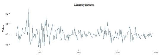
The EdhecRet function simply returns a ggplot of time series returns for the chosen strategy. The reason for storing these plots as elements of a list object is to simplify access to fund/regime results in the final dashboard of results. For example, to access the monthly return plot for Short.Selling strategy,edhec.ret$Short.Selling yields :

 

The code for that function is simply :

#########################################################################################
# Simple Fund Returns
#########################################################################################

EdhecRet <- function(xts.ret){
	loc <- environment()
	temp.df <- NULL
	temp.df <- data.frame(TimeIdx=as.Date(index(xts.ret)),coredata(xts.ret),stringsAsFactors=F)
	pp <- ggplot(data=temp.df,aes(x=TimeIdx,y=eval(parse(text=colnames(temp.df)))),environment=loc)+
						      theme_tufte(base_size=11)+
			            geom_line(size=0.5,color='skyblue4') +
			            labs(y='Values',title='Monthly Returns',x='')+
			        		theme(legend.position = "none")
	return(pp)
}
#########################################################################################

l
Now that we have downloaded or generated the necessary data series, the next posts shall deal with [1] fitting a 2 state hidden markov model to the economic regime variables and [2] assessing in-sample performance of different strategies across the hidden states for each regime variable. Ultimately I wish to present a dashboard of results for a chosen fund/regime combination.

• asset returns
• hidden markov model
• R
• regime switching